BigData 2018: Difference between revisions
imported>Weigang m (→Learning Goals) |
imported>Weigang |
||
| (42 intermediate revisions by the same user not shown) | |||
| Line 1: | Line 1: | ||
<center>'''Introduction to Evolutionary Genomics''' | <center>[http://bigdata.citytech.cuny.edu/ City Tech/Cornell BioMedical Big Data Week 2018]: '''Introduction to Evolutionary Genomics'''</center> | ||
<center>Thursday, June 21, 2018, 9-12</center> | |||
<center>'''Instructor:''' Dr Weigang Qiu, Associate Professor, Department of Biological Sciences </center> | <center>'''Instructor:''' Dr Weigang Qiu, Associate Professor, Department of Biological Sciences </center> | ||
<center>'''Office:''' B402 Belfer Research Building</center> | <center>'''Office:''' B402 Belfer Research Building</center> | ||
| Line 5: | Line 6: | ||
<center>'''Lab Website:''' http://diverge.hunter.cuny.edu/labwiki/</center> | <center>'''Lab Website:''' http://diverge.hunter.cuny.edu/labwiki/</center> | ||
---- | ---- | ||
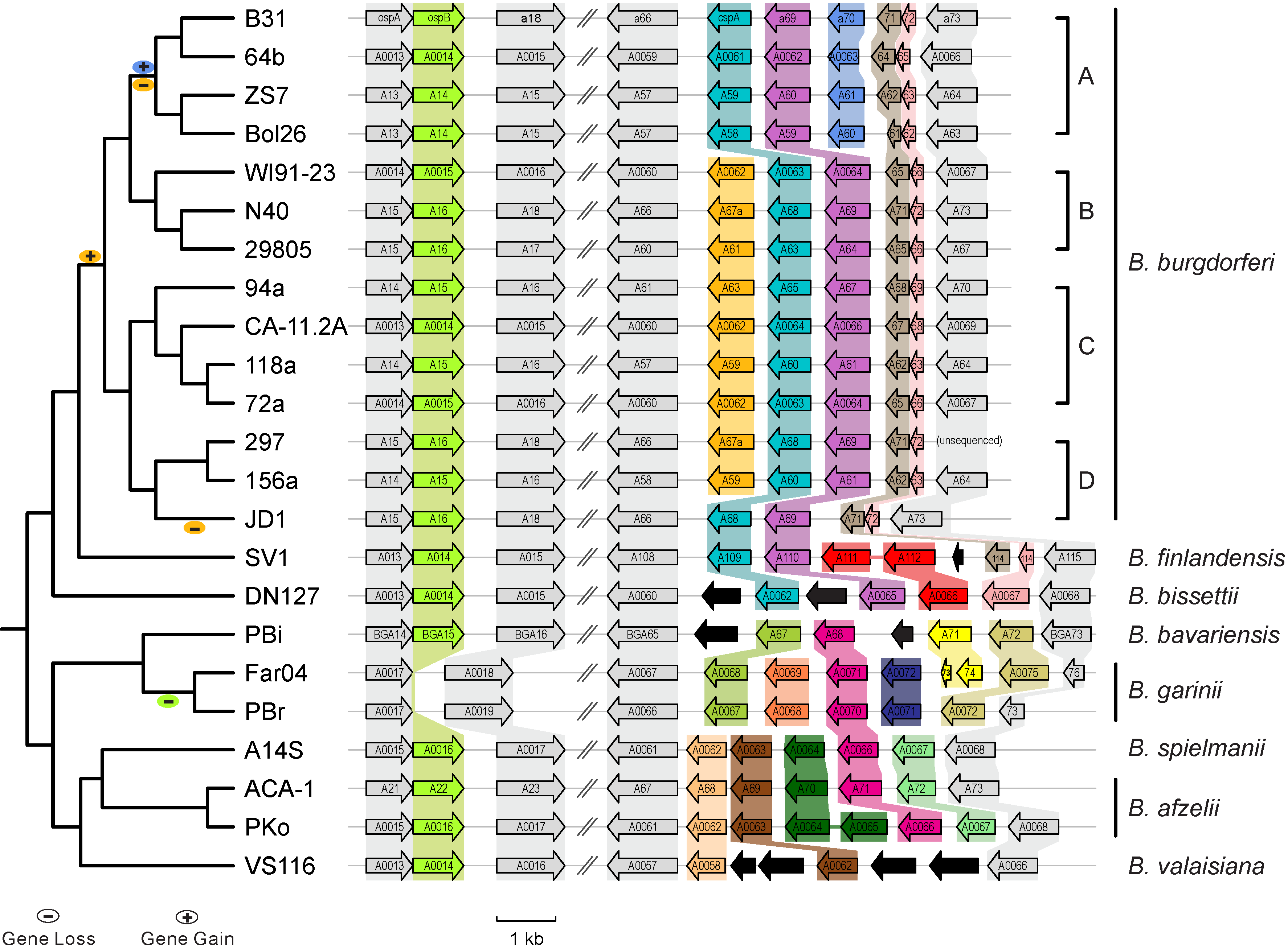
[[File: | [[File:Lp54-gain-loss.png|200px|thumbnail|Figure 1. Gains & losses of host-defense genes among Lyme pathogen genomes (Qiu & Martin 2014)]] | ||
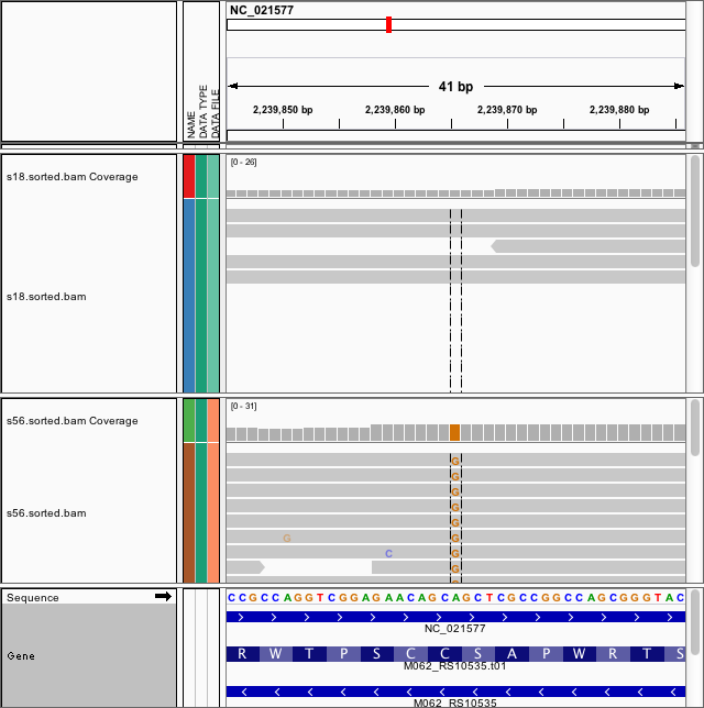
[[File:Igv mdpa.png|200px|thumbnail|Figure 2. Development of drug resistance mutation in Pseudomonas in a single cancer patient: top (April) vs. bottom (July) (Un-published data)]] | |||
==What is evolutionary genomics?== | ==What is evolutionary genomics?== | ||
Genomes differ among individuals and species. Evolutionary genomics studies genome variability and genome changes using evolutionary principles. Typical applications include identification of human genome variations associated with diseases and identification of pathogen virulence genes. | Genomes differ among individuals and species. Evolutionary genomics studies genome variability and genome changes using evolutionary principles. Typical applications include identification of human genome variations associated with diseases and identification of pathogen virulence genes. | ||
| Line 15: | Line 17: | ||
The key for comparing genomes across species is "tree-thinking", the idea that evolution happens by diversification (like a branching tree), not by climbing a ladder. There is no such thing as "advanced" or "primitive" species. All living species have the exact same evolutionary distances/time of divergence since the origin of life. | The key for comparing genomes across species is "tree-thinking", the idea that evolution happens by diversification (like a branching tree), not by climbing a ladder. There is no such thing as "advanced" or "primitive" species. All living species have the exact same evolutionary distances/time of divergence since the origin of life. | ||
== | ==Case studies from Qiu Lab== | ||
* Comparative genomics of worldwide Lyme disease pathogens | * Between-sepcies genome comparisons: Comparative genomics of worldwide Lyme disease pathogens. [http://borreliabase.org/ BorreliaBase] (Figure 1) | ||
* Evolution of multi-drug antibiotic-resistance Pseudomonas in cancer patients | * Within-population genome comparison: Genomic epidemiology of Group B Streptococcus: [http://diverge.hunter.cuny.edu/~weigang/gbs-browser/%20 Gene gains & losses associated with Group B Streptococcus virulence] | ||
* Within-host genome evolution: Evolution of multi-drug antibiotic-resistance Pseudomonas in cancer patients (Figure 2) | |||
== | ==Bioinformatics workflow for comparative analysis of bacterial pathogen genomes== | ||
* Pathogen isolation -> DNA extraction -> Library preparation -> High-through sequencing | |||
* De novo genome assembly (canu; velvet; etc) | |||
* Identify reference genome from NCBI database (kraken) | |||
* Variant call (bwa; cortex_var; samtools mpileup) | |||
* Infer genome phylogeny (muscle; reXML) | |||
* Annotation (PATRIC) | |||
* Custom genome browser (JavaScript; D3 library for interactive graphics) | |||
==Essential bioinformatics skills== | |||
* Linux command-line interface (e.g., BASH shell) | |||
* Familiarity with a programming language (e.g., Python or Perl) | |||
* Data visualization & statistical analysis (e.g., JavaScript; the R statistical computing environment) | |||
==Textbooks for genome evolution== | |||
* Graur, 2016, Molecular and Genome Evolution, First Edition, Sinauer Associates, Inc. ISBN: 978-1-60535-469-9. [http://www.sinauer.com/molecular-and-genome-evolution.html Publisher's Website] | * Graur, 2016, Molecular and Genome Evolution, First Edition, Sinauer Associates, Inc. ISBN: 978-1-60535-469-9. [http://www.sinauer.com/molecular-and-genome-evolution.html Publisher's Website] | ||
* Baum & Smith, 2013. Tree Thinking: an Introduction to Phylogenetic Biology, Roberts & Company Publishers, Inc. | * Baum & Smith, 2013. Tree Thinking: an Introduction to Phylogenetic Biology, Roberts & Company Publishers, Inc. | ||
| Line 29: | Line 45: | ||
* Be able to perform genome-wide association analysis on the R platform | * Be able to perform genome-wide association analysis on the R platform | ||
== | ==Schedule== | ||
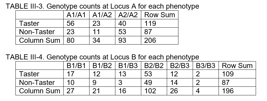
* "Tree | [[File:Taster-gene-tables.PNG|400px|thumbnail|Figure 3. Data sets for genotype-phenotype association tests]] | ||
* | |||
* 9:00 - 9:25: Introduction; [http://rstudio.org Install R & R Studio]; Download fasta file & save as "ospC-pep.fasta" : [[File:OspC-pep.txt|thumbnail]] | |||
* 9:30 - 10:00: Unix Tutorial ([http://korflab.ucdavis.edu/Unix_and_Perl/current.html#part1 Part I. Unix Basics]) | |||
* 10:05 - 10:30: Unix Tutorial ([http://korflab.ucdavis.edu/Unix_and_Perl/current.html#part2 Part II Advanced Unix]) | |||
* 10:35 - 11:00: Tree-thinking Quizzes: Slides [[File:Big-data-2018-phylogeny--slides.pptx|thumbnail]] & Handouts | |||
* 11:05 - 11:35: Test of genotype-phenotype association (Figure 3). | |||
<syntaxhighlight lang="bash"> | |||
geno.a <- matrix(c(53,20,39, 17, 9, 52), nrow = 2, byrow = T) | |||
geno.b <- matrix(c(13,10,11,49,9,1,12,5,1,38,10,1), nrow = 2, byrow = T) | |||
colnames(geno.a) <- c("A1A1", "A1/A2", "A2/A2") | |||
rownames(geno.a) <- c("Taster", "Non.Taster") | |||
rownames(geno.b) <- c("Taster", "Non.taster") | |||
colnames(geno.b) <- c("B1B1", "B1/B2", "B1/B3", "B2/B2", "B2/B3", "B3/B3") | |||
# plots | |||
mosaicplot(t(geno.a), cex.axis = 1, col = c("pink","cyan"), main = "Locus A") | |||
mosaicplot(t(geno.b), cex.axis = 1, col = c("pink","cyan"), main = "Locus B") | |||
# genotype-phenotype association | |||
test.geno.a <- chisq.test(geno.a) | |||
test.geno.b <- chisq.test(geno.b, simulate.p.value = T) | |||
</syntaxhighlight> | |||
* 11:40 - 12:00: Summary & Conclusion | |||
==Exercises & Challenges== | |||
* Finish Tree Thinking Quizzes | |||
* Unix exercises: | |||
** count the number of sequences using "grep -v" or "wc" | |||
** display the first 5 lines of a file | |||
** display the last 5 lines of a file | |||
** change upper-cases to lower-cases | |||
** change "|" to "_" | |||
** replace strings | |||
* R exercises: | |||
** Challenge: Test allele-phenotype association at two loci | |||
** [[R-tutorial|Exploration of human gene lengths using R]] | |||
Latest revision as of 06:07, 21 June 2018
What is evolutionary genomics?
Genomes differ among individuals and species. Evolutionary genomics studies genome variability and genome changes using evolutionary principles. Typical applications include identification of human genome variations associated with diseases and identification of pathogen virulence genes.
Genome changes are studied at two distinct levels: (1) within-species/within-population variations (e.g., human genetic variation), and (2) between-species divergence (e.g., human-mouse comparisons).
The key for analyzing genome variations within species is "population-thinking", the idea that there is no one individual genome that is standard, normal, or disease-free.
The key for comparing genomes across species is "tree-thinking", the idea that evolution happens by diversification (like a branching tree), not by climbing a ladder. There is no such thing as "advanced" or "primitive" species. All living species have the exact same evolutionary distances/time of divergence since the origin of life.
Case studies from Qiu Lab
- Between-sepcies genome comparisons: Comparative genomics of worldwide Lyme disease pathogens. BorreliaBase (Figure 1)
- Within-population genome comparison: Genomic epidemiology of Group B Streptococcus: Gene gains & losses associated with Group B Streptococcus virulence
- Within-host genome evolution: Evolution of multi-drug antibiotic-resistance Pseudomonas in cancer patients (Figure 2)
Bioinformatics workflow for comparative analysis of bacterial pathogen genomes
- Pathogen isolation -> DNA extraction -> Library preparation -> High-through sequencing
- De novo genome assembly (canu; velvet; etc)
- Identify reference genome from NCBI database (kraken)
- Variant call (bwa; cortex_var; samtools mpileup)
- Infer genome phylogeny (muscle; reXML)
- Annotation (PATRIC)
- Custom genome browser (JavaScript; D3 library for interactive graphics)
Essential bioinformatics skills
- Linux command-line interface (e.g., BASH shell)
- Familiarity with a programming language (e.g., Python or Perl)
- Data visualization & statistical analysis (e.g., JavaScript; the R statistical computing environment)
Textbooks for genome evolution
- Graur, 2016, Molecular and Genome Evolution, First Edition, Sinauer Associates, Inc. ISBN: 978-1-60535-469-9. Publisher's Website
- Baum & Smith, 2013. Tree Thinking: an Introduction to Phylogenetic Biology, Roberts & Company Publishers, Inc.
Learning Goals
- Be able to compare evolutionary relationships using phylogenetic trees
- Be able to use command-line tools for batch-processing of genome files
- Be able to perform genome-wide association analysis on the R platform
Schedule
- 9:00 - 9:25: Introduction; Install R & R Studio; Download fasta file & save as "ospC-pep.fasta" :
- 9:30 - 10:00: Unix Tutorial (Part I. Unix Basics)
- 10:05 - 10:30: Unix Tutorial (Part II Advanced Unix)
- 10:35 - 11:00: Tree-thinking Quizzes: Slides & Handouts
- 11:05 - 11:35: Test of genotype-phenotype association (Figure 3).
geno.a <- matrix(c(53,20,39, 17, 9, 52), nrow = 2, byrow = T)
geno.b <- matrix(c(13,10,11,49,9,1,12,5,1,38,10,1), nrow = 2, byrow = T)
colnames(geno.a) <- c("A1A1", "A1/A2", "A2/A2")
rownames(geno.a) <- c("Taster", "Non.Taster")
rownames(geno.b) <- c("Taster", "Non.taster")
colnames(geno.b) <- c("B1B1", "B1/B2", "B1/B3", "B2/B2", "B2/B3", "B3/B3")

# plots
mosaicplot(t(geno.a), cex.axis = 1, col = c("pink","cyan"), main = "Locus A")
mosaicplot(t(geno.b), cex.axis = 1, col = c("pink","cyan"), main = "Locus B")

# genotype-phenotype association
test.geno.a <- chisq.test(geno.a)
test.geno.b <- chisq.test(geno.b, simulate.p.value = T)
- 11:40 - 12:00: Summary & Conclusion
Exercises & Challenges
- Finish Tree Thinking Quizzes
- Unix exercises:
- count the number of sequences using "grep -v" or "wc"
- display the first 5 lines of a file
- display the last 5 lines of a file
- change upper-cases to lower-cases
- change "|" to "_"
- replace strings
- R exercises:
- Challenge: Test allele-phenotype association at two loci
- Exploration of human gene lengths using R


