Biol375 2019: Difference between revisions
imported>Lab m (change package spelling to phangorn) |
imported>Weigang |
||
| Line 298: | Line 298: | ||
* 12/2 (M). SNP statistics & gene frequency analysis: In-class exercises. | * 12/2 (M). SNP statistics & gene frequency analysis: In-class exercises. | ||
* 12/5 (TH) Genetic Drift (pages 47-49). Lecture slides: [[File:Part-4-evol-mechanism-2018.pdf|thumbnail]] | * 12/5 (TH) Genetic Drift (pages 47-49). Lecture slides: [[File:Part-4-evol-mechanism-2018.pdf|thumbnail]] | ||
* 12/9 (M). (Last Lecture) Review & Course evaluations. Final review slides: [[File:Final-review- | * 12/9 (M). (Last Lecture) Review & Course evaluations. Final review slides: [[File:Final-review-2019.pdf|thumbnail]] | ||
** '''Submit your Teacher's Evaluation''', using either: | ** '''Submit your Teacher's Evaluation''', using either: | ||
** Personal computer at [http://www.hunter.cuny.edu/te www.hunter.cuny.edu/te]; or, | ** Personal computer at [http://www.hunter.cuny.edu/te www.hunter.cuny.edu/te]; or, | ||
** Smartphone at [http://www.hunter.cuny.edu/mobilete www.hunter.cuny.edu/mobilete] | ** Smartphone at [http://www.hunter.cuny.edu/mobilete www.hunter.cuny.edu/mobilete] | ||
* Dec 16 (Monday) 4-6pm: '''Comprehensive Final Exam''' | * Dec 16 (Monday) 4-6pm: '''Comprehensive Final Exam''' | ||
Latest revision as of 16:37, 9 December 2019
Course Description
Molecular evolution is the study of the change of DNA and protein sequences through time. Theories and techniques of molecular evolution are widely used in species classification, biodiversity, comparative genomics, and molecular epidemiology. Contents of the course include:
- Population genetics, which is a theoretical framework for understanding mechanisms of sequence evolution through mutation, recombination, gene duplication, genetic drift, and natural selection.
- Molecular systematics, which introduces statistical models of sequence evolution and methods for reconstructing species phylogeny.
- Bioinformatics, which provides hands-on training on data acquisition and the use of software tools for phylogenetic analyses.
This 3-credit course is designed for upper-level biology-major undergraduates. Hunter pre-requisites are BIOL203, and MATH150 or STAT113.
Textbooks
- (Required) Graur, 2016, Molecular and Genome Evolution, First Edition, Sinauer Associates, Inc. ISBN: 978-1-60535-469-9. Publisher's Website (Student discount: a 15% discount and receive free UPS standard shipping)
http://www.sinauer.com/molecular-and-genome-evolution.html)
- (Recommended) Baum & Smith, 2013. Tree Thinking: an Introduction to Phylogenetic Biology, Roberts & Company Publishers, Inc.
Learning Goals
- Be able to describe evolutionary relationships using phylogenetic trees
- Be able to use web-based as well as stand-alone software to infer phylogenetic trees
- Understand mechanisms of DNA sequence evolution
- Understand algorithms for building phylogenetic trees
Links for phylogenetic tools
- NCBI sequence databases
- R Tools
- R source: download & install from a mirror site
- R Studio: download & install
- APE package
- phangorn package
- A Molecular Phylogeny Web Server
- EvolView: an online tree viewer
Exams & Grading
- Bonus for full attendance & active participation in classroom discussions.
- Assignments. All assignments should be handed in as hard copies only. Email submission will not be accepted. Late submissions will receive 10% deduction (of the total grade) per day.
- Three Mid-term Exams (30 pts each)
- Comprehensive Final Exam (50 pts)
Academic Honesty
While students may work in groups and help each other for assignments, duplicated answers in assignments will be flagged and investigated as possible acts of academic dishonesty. To avoid being investigated as such, do NOT copy anyone else's work, or let others copy your work. At the least, rephrase using your own words. Note that the same rule applies regarding the use of textbook and online resources: copied sentences are not acceptable and will be considered plagiarism.
Hunter College regards acts of academic dishonesty (e.g., plagiarism, cheating on examinations, obtaining unfair advantage, and falsification of records and official documents) as serious offenses against the values of intellectual honesty. The College is committed to enforcing the CUNY Policy on Academic Integrity and will pursue cases of academic dishonesty according to the Hunter College Academic Integrity Procedures.
Course Schedule
Part 1. Tree Thinking
- 8/29 (TH). Overview & Introduction. Textbook Chapter: "Introduction" (pages 1-3)
| Assignment 1 (10 pts; Due next class 9/5) |
|---|
|
- 9/5 (TH). Introduction (Continued)
- R terminologies
- Object: variable that contains data (e.g., "iris")
- Object class: type of data (e.g., "data.frame", which is a table)
- Function: e.g., data(iris), which loads the data set called "iris"
- Function arguments: input and options (e.g., "iris" above)
- Tutorial: R & R-Studio (Bring your own computer)
- Lecture slides:
- R terminologies
| Assignment 2 (5 pts; Due: next session) |
|---|
R exercises
|
- 9/9 (M). Intro to trees
- Go over pre-test questions
- In-class exercise 1 (5 pts)
- Introduction to tree
- 9/12 (TH). Intro to trees (continued)
- In-class exercise 2. (5 pts)
- Textbook Chapter 5: "Molecular Phylogenetics" (pages 170-175; 201-202)
- 9/16 (M). Species Tree & Lineage Sorting.
- Textbook Chapter 5: "Molecular Phylogenetics" (pages 177-180).
- 9/19 (TH). Consensus Tree & Review.
- Chapter 5. pages 199-200 (Figure 5.31)
- In-class exercise 3. (5 pts, due next session)
- Lecture Slides:
- 9/23 (M). 4:10 - 5:10pm Midterm Exam I Bring pencils, erasers, and a calculator
Part 2. Analysis of Trait Evolution
- 9/26 (TH). Traits & trait matrix
- Textbook Chapter 5, pages 180-183
- R demo I (by Chris)
# iris dataset exercise
# load libraries
library(tidyverse)
library(datasets)
data('iris')

# summary of data
summary(iris)
glimpse(iris)
iris %>% glimpse()

# previewing data
head(iris)

# subsetting data
slice(iris, 1:3)
iris %>% slice(1:3)

# grouping and subsetting data
iris %>%
  group_by(Species) %>%
  slice(1:3)

iris %>%
  group_by(Species) %>%
  summarise(average = mean(Sepal.Length))

# filtering data
filter(iris, Species == 'versicolor')
iris %>%
  filter(Species == 'versicolor')

iris %>%
  filter(Sepal.Length >= 7)

# OR operation
iris %>%
  filter(Sepal.Length < 5 | Sepal.Length > 7)

# check distribution using histogram
ggplot(iris, aes(x = Sepal.Length)) +
  geom_histogram()

# distribution by Species
ggplot(iris, aes(x = Sepal.Length, fill = Species)) +
  geom_histogram(alpha = 0.5)

# distribution by Species using facetwrap
ggplot(iris, aes(x = Sepal.Length, color = Species)) +
  geom_histogram() + facet_wrap(~Species)

# boxplot
ggplot(iris, aes(y = Sepal.Length, x = Species)) +
  geom_boxplot()

# boxplot with points
ggplot(iris, aes(y = Sepal.Length, x = Species)) +
  geom_boxplot() +
  geom_jitter(size = 2, width = 0.1, alpha = 0.5, color = 'blue')

# scatterplot
ggplot(iris, aes(y = Sepal.Length, x = Petal.Length, color = Species)) + geom_point()
| Assignment #3 (5 pts; Due next session) |
|---|
Watch Origin of Species: Lizards in an Evolutionary Tree. Provide short answer (1-3 sentences) to each of the following three questions.
|
- 10/3 (TH). Homoplasy & consistency
- Character & Character states
- R Demo (part 2) (Crhis)
| Bonus R Exercise (10 pts; Due 10/10, Thursday) |
|---|
|
- 10/7 (M). Parsimony reconstruction (Chapter 5).
- Textbook Chapter 5, pages 188-191
| Assignment #4 (5 pts; Due next session) |
|---|
|
- 10/10 (TH). Parsimony reconstruction (Continued)
- In-Class Exercise 4
- Lecture slides:
- 10/16 (Wed. Monday Schedule). Genome & gene structure (Chapter 3)
- Calculate consistency indices for lizard ecomorphs & geographic orgins
- | Graur et al (2013). "On the immotality of television sets"
- 10/17 (TH). Review & Practices.
- In-class exercise: hemoglobin gene structure
- In-Class Exercise: Pretest Part 2,
- 10/21 (M). Midterm Exam 2
Part 3. Tree Algorithms
- 10/24 (TH). (No Class)
- 10/28 (M).
- BLAST & Alignments (Chapter 3. pages 93-100).In-class exercise: Run BLAST; show alignment & explain E-value
- Genetic distances
- 10/31 (TH).
- Sequence-evolutionary models (Chapter 3, pages 79-88). In-class exercise: Poisson simulation & explain
- Lecture slides:
- 11/4 (M).
- Distance methods (Chapter 5, pages 184-187). In class exercise: use APE package to calculate genetic distances
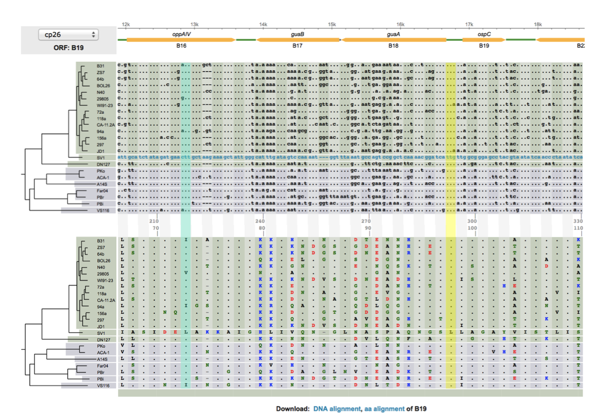
- In class exercise: calculate Jukes-Cantor distance of this DNA sequence alignment. Note: Ignore gapped positions.
- 11/7 (TH).
- Maximum parsimony (Chapter 5, pages 191-194). In-class exercise: parsimony scores
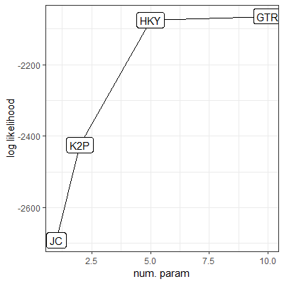
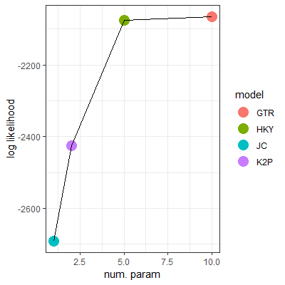
- Likelihood & Bayesian methods;
- Bonus assignment II (5 pts, Due 11/18, Monday):
|
- 11/11 (M).
- Tree Testing (Chapter 5, pages 194-198).
- 11/14 (TH).
- Review exercises (Chapter 5, pages 207-209) .
- 11/18 (M). 3rd Mid-term exam
Part 4. Mechanisms of molecular evolution
- 11/21 (TH).
- Mechanism of molecular evolution: Overview (pages 35-38) & Rates of nucleotide substitutions (pages 111-125).
- 11/25 (M). In-class computer exercise:
- Ka/Ks test of natural selection (pg 116-124). In-class exercise
| Final project (20 pts). Due: 12/9, Monday) |
|---|
|
- 12/2 (M). SNP statistics & gene frequency analysis: In-class exercises.
- 12/5 (TH) Genetic Drift (pages 47-49). Lecture slides:
- 12/9 (M). (Last Lecture) Review & Course evaluations. Final review slides:
- Submit your Teacher's Evaluation, using either:
- Personal computer at www.hunter.cuny.edu/te; or,
- Smartphone at www.hunter.cuny.edu/mobilete
- Dec 16 (Monday) 4-6pm: Comprehensive Final Exam


