Southwest-University: Difference between revisions
imported>Weigang |
imported>Lia |
||
| Line 204: | Line 204: | ||
* Dataset: [[File:Cancer-array.txt|thumbnail]] (provided by Prof Zhu) | * Dataset: [[File:Cancer-array.txt|thumbnail]] (provided by Prof Zhu) | ||
* Quiz II. | * Quiz II. | ||
* Code for MA plot (by Dr Di) | |||
<syntaxhighlight> | <syntaxhighlight> | ||
# Cancer microarray dataset (Data provided by Prof. Zhu) | # Cancer microarray dataset (Data provided by Prof. Zhu) | ||
| Line 231: | Line 226: | ||
ggplot(arr.fc, aes(x=control+treat, y=fc, color=fc)) + theme_bw() + geom_point(size=0.5) + scale_color_gradient2(midpoint=0, low="blue", mid="gray", high="red") + xlab("Total Expression") + ylab("Fold Change") + geom_hline(yintercept = c(-1, 0, 1), linetype="dashed") | ggplot(arr.fc, aes(x=control+treat, y=fc, color=fc)) + theme_bw() + geom_point(size=0.5) + scale_color_gradient2(midpoint=0, low="blue", mid="gray", high="red") + xlab("Total Expression") + ylab("Fold Change") + geom_hline(yintercept = c(-1, 0, 1), linetype="dashed") | ||
</syntaxhighlight> | </syntaxhighlight> | ||
[[File:GeneExp1.jpeg|400px|thumbnail|heatmap for cancer microarray]] | |||
* Code for t-test | |||
<syntaxhighlight> | |||
# 4. run t-tests for each gene | # 4. run t-tests for each gene | ||
library(broom) | library(broom) | ||
| Line 240: | Line 236: | ||
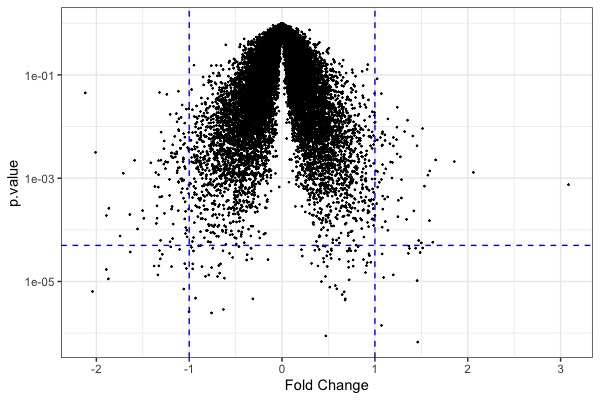
ggplot(t.model, aes(x=estimate, y=p.value)) + geom_point(size=0.2) + scale_y_log10() + geom_hline(yintercept = 5e-5, color="blue", linetype="dashed") + geom_vline(xintercept = c(-1,1), color="blue", linetype="dashed") + xlab("Fold Change") + theme_bw() # volcano plot | ggplot(t.model, aes(x=estimate, y=p.value)) + geom_point(size=0.2) + scale_y_log10() + geom_hline(yintercept = 5e-5, color="blue", linetype="dashed") + geom_vline(xintercept = c(-1,1), color="blue", linetype="dashed") + xlab("Fold Change") + theme_bw() # volcano plot | ||
</syntaxhighlight> | </syntaxhighlight> | ||
[[File:GeneExp2.jpeg|400px|thumbnail|Vocalno plot for cancer microarray]] | [[File:GeneExp2.jpeg|400px|thumbnail|Vocalno plot for cancer microarray]] | ||
* Code for heatmap | |||
<syntaxhighlight> | <syntaxhighlight> | ||
# 5. select & plot significant genes | # 5. select & plot significant genes | ||
| Line 253: | Line 249: | ||
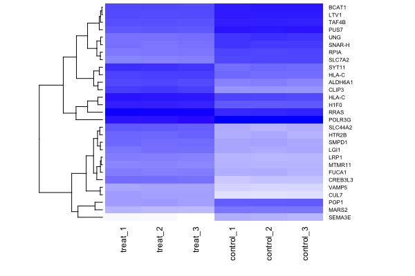
heatmap(arr.mat, cexRow = 0.6, cexCol = 0.9, scale="none", col=colorpanel(360,"white","blue"), Colv = NA) | heatmap(arr.mat, cexRow = 0.6, cexCol = 0.9, scale="none", col=colorpanel(360,"white","blue"), Colv = NA) | ||
</syntaxhighlight> | </syntaxhighlight> | ||
[[File:GeneExp3.jpeg|400px|thumbnail|heatmap for cancer microarray]] | |||
===Session 8. Final presentation=== | ===Session 8. Final presentation=== | ||
Revision as of 10:24, 20 July 2019
Professor, Department of Biological Sciences, City University of New York, Hunter College & Graduate Center
Adjunct Faculty, Department of Physiology and Biophysics, Institute for Computational Biomedicine, Weil Cornell Medical College
Associate Professor, School of Life Science, South West University
Course Overview
Welcome to BioMedical Genomics, a computer workshop for advanced undergraduates and graduate students. A genome is the total genetic content of an organism. Driven by breakthroughs such as the decoding of the first human genome and next-generation DNA -sequencing technologies, biomedical sciences are undergoing a rapid and irreversible transformation into a highly data-intensive field.
Genome information is revolutionizing virtually all aspects of life sciences including basic research, medicine, and agriculture. Meanwhile, use of genomic data requires life scientists to be familiar with concepts and skills in biology, computer science, as well as data analysis.
This workshop is designed to introduce computational analysis of genomic data through hands-on computational exercises, using published studies.
The pre-requisites of the course are college-level courses in molecular biology, cell biology, and genetics. Introductory courses in computer programming and statistics are preferred but not strictly required.
Learning goals
By the end of this course successful students will be able to:
- Describe next-generation sequencing (NGS) technologies & contrast it with traditional Sanger sequencing
- Explain applications of NGS technology including pathogen genomics, cancer genomics, human genomic variation, transcriptomics, meta-genomics, epi-genomics, and microbiome.
- Visualize and explore genomics data using RStudio
- Replicate key results using a raw data set produced by a primary research paper
Web Links
- Install R base: https://cloud.r-project.org
- Install R Studio (Desktop version): http://www.rstudio.com/download
- Download: R datasets
- A reference book: R for Data Science (Wickharm & Grolemund)
Quizzes and Exams
Student performance will be evaluated by attendance, three (4) quizzes and a final report:
- Attendance: 50 pts
- Assignments: 5 x 10 = 50 pts
- Open-book Quizzes: 2 x 25 pts = 50 pts
- Take-home Mid-term: 50 pts
- Final presentation: 50 pts
Total: 250 pts
Course Schedule
Session 1. Introduction & R Tutorial I
- Date & Hours: July 8 (Mon), 8:40-12:10
- Lecture slides: File:R-part-1-small.pdfLecture slides
- Assignment #1 (create a WORD document including scripts & graphs (i.e., compile your work into a lab report, due tomorrow)
- Install R/R studio and the "tidyverse" package on your own computer
- Recreate Script 1 & Mini-Practical
- Show help page for function "seq"
- Download dataset
- Create a new folder (e.g., Desktop/rtutor)
- Create a sub-folder (e.g., Desktop/rtutor/data/)
- Download from http://www.r4all.org/the-book/datasets
- Save to the sub-folder
- Unzip the file
Session 2. R Tutorial II
- Date & Hours: July 9 (Tu), 8:40-12:10
- Lecture slides: File:R-part-2.pdfLecture slides
- Assignment #2.
The following is a portion of the dataset of Mycobacterium growth (kindly shared by Aswad from Dr Xie's lab). It shows OD (optical density) values. Transform this table ("wide" format) into the "tall/tidy" format (use paper & pen, no need to use R studio or any computer program):
| Hour | Control | Gene | Control.with.Arg | Gene.with.Arg |
|---|---|---|---|---|
| 0 | 0.06 | 0.022 | 0.031 | 0.01 |
| 4 | 0.087 | 0.102 | 0.082 | 0.081 |
| 8 | 0.113 | 0.185 | 0.086 | 0.135 |
- In R studio, read the dataset from the file "FlowerColourVisits.csv" and save it into an object named as "flower"
- Show head, tail, dimension of the data frame "flower"
- Show data summary with "summary" & "glimpse" commands. Which column is a categorical data type?
- Select the column named "colour"
- Select rows from the 3rd to the 20th
- Select the 3rd, 10th, and 20th rows
- Select only the rows that have the colour of "red" (hint use
colour=="red" - Create a new column, named "logVisit", that is log(1+number.of.visit)
- Sort the "flower" data by the column "number.of.visit"
- Perform the following data transformation using the chaining operator (i.e., "%>%"): Select rows from the 3rd to the 20th, then filter by colour of "red", and then show head
- Obtain the mean number of visit for each colour as a group (Hint: use "group_by" & "summarise")
Session 3. R Tutorial III & Quiz I
- Date & Hours: July 10 (Wed), 8:40-12:10
- Lecture slides: File:R-part-3.pdfLecture slides
- Assignment #3
| Task | Graph |
|---|---|
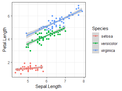
Use the "iris" dataset to reproduce the plot shown at right (Hint: load data with data(iris)) |
|
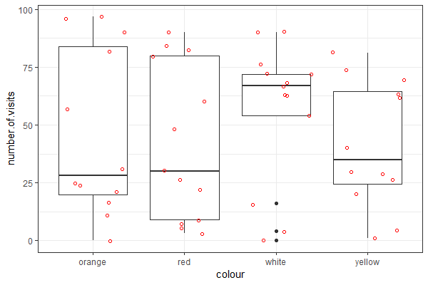
| Use the "flower" dataset (see Assignment #2 on how to load data) to reproduce the plot shown at right |
Session 4. Intro to NGS & R Tutorial IV
- Date & Hours: July 11 (Thur), 8:40-12:10
- Slides for NGS:
- Slides for R Tutorial IV; File:R-part-4.pdfLecture slides
- Take-home mid-term (50 pts)
Weekend break (No class; July 12 - 14, Fri, Sat & Sun)
Session 5. Case Study I (Trout microbiome) & R Tutorial V
- Date & Hours: July 15 (Mon), 8:30-12:10
- Dataset:
- Slides for R Tutorial Part V: File:R-part-5.pdfLecture slides
- Slide for trout microbiome: File:Case-1-Trout-Microbiome.pdfLecture slides
R code for today's lecture
# Case Study 1. Trout microbiome
# Date: Monday, July 15, 2019
# Author: Weigang Qiu

library(tidyverse)
# Load data
setwd("C:/Users/lai/Dropbox/Courses/ChongQing-2019/")

trout <- read_csv("Trout.txt")
glimpse(trout)

# Exercise 1. Transform into a long table
trout.long <- gather(trout, 2:29, key = "sample", value = "read.cts")

# Exercise 2. filter out phyla < 1%
trout.ph.cts <- trout.long %>% group_by(phylum) %>% summarise(phy.sum = sum(read.cts)) # counts in each phylum
trout.ph.perc <- trout.ph.cts %>% mutate(ph.perc = phy.sum/sum(phy.sum) * 100) # get percentages
trout.ph.hi <- trout.ph.perc %>% filter(ph.perc > 1) # select phyla > 1%

# The above could be combined using pipes
# trout.ph.hi <- trout.long %>% group_by(phylum) %>% summarise(cts = sum(read.cts)) %>% mutate(perc = cts/sum(cts) * 100) %>% filter(perc >= 1)

# Exercise 3. get phylum counts in each sample
trout.ph <- trout.long %>% filter(phylum %in% trout.ph.hi$phylum) # select only the hi-frequency phyla
trout.ph <- trout.ph %>% group_by(sample, phylum) %>% summarise(total.cts = sum(read.cts)) # counts in each sample
trout.ph <- trout.ph %>% mutate(per.cts = total.cts/sum(total.cts) * 100) # add perc
trout.ph %>% group_by(sample) %>% summarise(sum(per.cts)) # check

# Exercise 4. plot by sample
ggplot(data = trout.ph, aes(x=sample, y=per.cts, fill=phylum)) + geom_bar(stat = 'identity')

# Exercise 5. group by diet
trout.ph <- trout.ph %>% mutate(diet = str_remove(sample, "_[1234]")) # add a new column "diet" use regular expression
trout.diet <- trout.ph %>% group_by(diet, phylum) %>% summarise(cts.by.diet = sum(total.cts)) %>% mutate(per.by.diet = cts.by.diet/sum(cts.by.diet)*100)
trout.diet %>% group_by(diet) %>% summarise(sum(per.by.diet)) # check
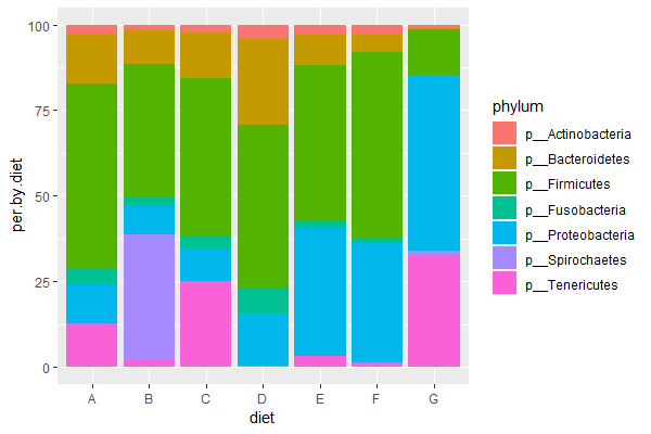
ggplot(data = trout.diet, aes(x=diet, y=per.by.diet, fill=phylum)) + geom_bar(stat = 'identity') # per, stacked
Assignment #4 (finalized at 8:25pm)
| 1. Define microbiome | |
| 2. Explain how 16S ribosomal RNA read counts are used to quantify bacterial composition | |
| 3. Run the above code (or your own code) & compose a figure legend explaining the final graph (explain x-axis, y-axis, and what colors represent). Which diet is most similar to the control diet ("E")? |
Session 6. Case Study 1. Trout microbiome (continued)
- Date & Hours: July 16 (Tu), 8:30-12:10
- Dataset:
- Today's code:
# Calculate alpha diversity (at species level)
trout <- read_csv("Trout.txt")
trout.long <- gather(trout, 2:29, key = "sample", value = "read.cts") # tranform into a long table
trout.long <- trout.long %>% mutate(diet = str_remove(sample, "_[1234]")) # add diet group variable
trout.sp <- trout.long %>% group_by(diet, species) %>% summarise(total.cts = sum(read.cts)) # count species reads in each diet
trout.sp2 <- trout.sp %>% filter(species != 's__') %>% filter(total.cts > 0) # remove species with un-specified & zeros reads
trout.sp2 %>% group_by(diet) %>% count() # count num. species per diet
trout.sp2 <- trout.sp2 %>% group_by(diet) %>% mutate(frq = total.cts/(sum(total.cts))) %>% mutate(log.frq = log2(frq)) # add columns for frequency and its log2()
trout.sp2 %>% group_by(diet) %>% summarise(-sum(frq * log.frq)) # shannon = -sum(p*log2(p)) # Shannon diversity for each diet

# ANOVA to compare two phyla: Fusobacteria and Bacteroidetes (beta-diversity)
trout <- read_csv("Trout.txt")
trout.long <- gather(trout, 2:29, key = "sample", value = "read.cts") # tranform into a long table
trout.ph <- trout.long %>% group_by(sample, phylum) %>% summarise(cts = sum(read.cts)) # count reads for each phylum in each sample
trout.ph <- trout.ph %>% group_by(sample) %>% mutate(perc = cts/sum(cts) *100) # calculate percentages
trout.fuso <- trout.ph %>% filter(phylum == 'p__Fusobacteria') # select rows for a phylum
trout.fuso <- trout.fuso %>% mutate(diet = str_remove(sample, "_[1234]")) # add diet
ggplot(data = trout.fuso, aes(x=diet, y=perc, color=diet)) +  geom_point(size=3, alpha=0.5) + theme_bw() # plot
lm.fuso <- lm(data = trout.fuso, perc ~ diet) # run anova model
summary(lm.fuso) # show difference with reference ("dietA") and p values
anova(lm.fuso) # show overall signficance

mean.fuso <- trout.fuso %>% group_by(diet) %>% summarise(mean.prc = mean(perc)) # calculate mean percentages for each diet
ggplot(data = trout.fuso, aes(x=diet, y=perc, color=diet)) +  geom_point(size=3, alpha=0.5) + geom_point(data = mean.fuso, aes(x=diet, y=mean.prc), shape = 10, size=6) + theme_bw() # add mean values

# Make diet E the reference:
trout.fuso <- trout.fuso %>% mutate(diet.mod = ifelse(diet=='E', str_c("control", diet), str_c("treat", diet)))
lm.fuso.mod <- lm(data = trout.fuso, perc ~ diet.mod)
summary(lm.fuso.mod)
- Assignment #5 (finalized @5:00pm)
- Run ANOVA to test if the percentages for the phylum "Bacteroidetes" are significantly different among the 7 diets.
- Show graph with mean percentages values
Session 7. Case Study 2. Cancer microarray
- Date & Hours: July 17 (Wed), 8:30-12:10
- Dataset: (provided by Prof Zhu)
- Quiz II.
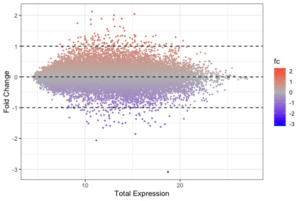
- Code for MA plot (by Dr Di)
# Cancer microarray dataset (Data provided by Prof. Zhu)
# July 10, 2019
# Weigang Qiu
library(tidyverse) # load library
setwd("C:/Users/lai/Dropbox/Courses/ChongQing-2019/")

# 1. Load data & make long table
arr <- read_csv(file = "Cancer-array.txt")
arr.long <- arr %>% gather(3:8, key = "control.treat", value = "gene.expression")
arr.long <- arr.long %>% mutate(group = str_remove(control.treat, "_[123]")) # create a treat/control variable
ggplot(data = arr.long, aes(x = control.treat, y=gene.expression, fill = group)) + geom_violin() # show distribution & density; normalized & already in log2()

# 2. calculate fold change
arr.fc <- arr.long %>% group_by(aff.id, group) %>% summarise(mean.exp = mean(gene.expression))
arr.fc <- arr.fc %>% spread(group, mean.exp)
arr.fc <- arr.fc %>% mutate(fc = treat-control)

# 3. MA plot, colored by fold change
ggplot(arr.fc, aes(x=control+treat, y=fc, color=fc)) + theme_bw() + geom_point(size=0.5) + scale_color_gradient2(midpoint=0, low="blue", mid="gray", high="red") + xlab("Total Expression") + ylab("Fold Change") + geom_hline(yintercept = c(-1, 0, 1), linetype="dashed")- Code for t-test
# 4. run t-tests for each gene
library(broom)
t.model <- arr.long %>% group_by(aff.id) %>% do(tidy(t.test(gene.expression ~ group, data = .))) # run t-test for each gene

ggplot(t.model, aes(x=estimate, y=p.value)) + geom_point(size=0.2) + scale_y_log10() + geom_hline(yintercept = 5e-5, color="blue", linetype="dashed") + geom_vline(xintercept = c(-1,1), color="blue", linetype="dashed") + xlab("Fold Change") + theme_bw() # volcano plot- Code for heatmap
# 5. select & plot significant genes
mod.select <- t.model %>% filter(p.value < 1e-4) # select significant genes
arr.sig <- arr %>% filter(aff.id %in% mod.select$aff.id)
arr.mat <- as.matrix(arr.sig[,3:8])
rownames(arr.mat) <- arr.sig$gene.symbol
library(gplots)
heatmap(arr.mat, cexRow = 0.6, cexCol = 0.9, scale="none", col=colorpanel(360,"white","blue"), Colv = NA)Session 8. Final presentation
- Date & hours: July 18 (Thur), 8:30-12:10
- Hints to prepare the final presentation:
- Use the trout microbiome dataset
- Show distributions of class/order/family/genus for each diet (we did it for the phylum in class)
- Calculate Shannon indices for phylum/class/order/family/genus in each diet (we did it for the species in class)
- Select a particular phylum/class/order/family/genus/species & test significance in percentages among diets using ANOVA (we did it for the phylum Fusobacteria in class
- Rubric for tinal presentations (4 slides, 5 minute)
- Slide 1. (1 min; 5 pts). Introduction: background, question, & signficance
- Slide 2. (1 min; 10 pts). Material & Methods: sample size, replicates, control, sequencing technology, software tools, statistical analysis
- Slide 3. (2 min; 15 pts). Results: a graph: title, legends, caption, main R commands
- Slide 4. (1 min; 5 pts). Discussion, conclusion & questions
- Slide style (10 pts). Use more figures, less words; show bullets & outlines, not complete sentences
- Presentation style (5 pts). Speak loudly, slowly, and clearly. Do not read from slides.
Papers & Datasets
| Omics Application | Paper link | Data set | NGS Technology |
|---|---|---|---|
| Microbiome | Rimoldi_etal_2018_PlosOne | 16S rDNA amplicon sequencing | |
| Transcriptome | Wang_etal_2015_Science | Tables S2 & S4 | RNA-Seq |
| Transcriptome & Regulome | Nava_etal_2019_BMCGenomics | Tables S2 & S3 | RNA-Seq & CHIP-Seq |
| Proteome | Qiu_etal_2017_NPJ | (to be posted) | SILAC |
| Population genomics (Lyme) | Di_etal_2018_JCM | Data & R codes | Amplicon sequencing (antigen locus) |
| Population genomics/GWAS (Human) | Simonti_etal_2016_Science | Table S2 | whole-genome sequencing (WGS); 1000 Genome Project (IGSR) |
| TB surveillance | Brow_etal_2015 | Sequence Archives | Whole-genome sequencing (WGS) |
