NYRaMP-Informatics-2025: Difference between revisions
| Line 399: | Line 399: | ||
==Demo. Microbiome data analysis== | ==Demo. Microbiome data analysis== | ||
* Mock gene expression data set: | * Mock gene expression data set: [[File:sample_gene_exp_dataset.csv|thumb]] | ||
* DNA barcoding dataset: | * DNA barcoding dataset, NYC soil microbiome [[File:abundance_table_species.tsv|thumb]] | ||
<syntaxhighlight lang='bash'> | <syntaxhighlight lang='bash'> | ||
library(tidyverse) | library(tidyverse) | ||
Revision as of 15:45, 20 August 2025
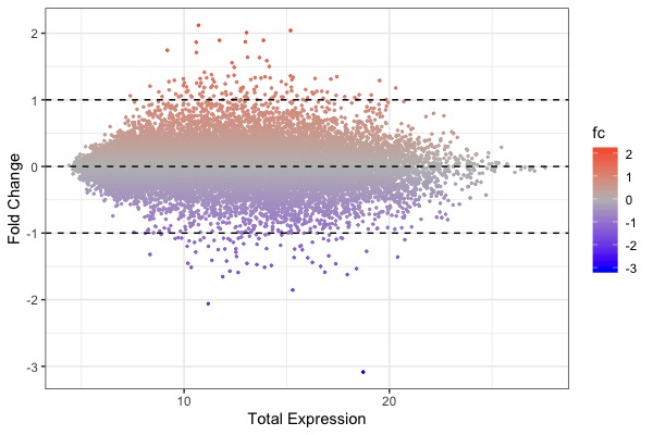
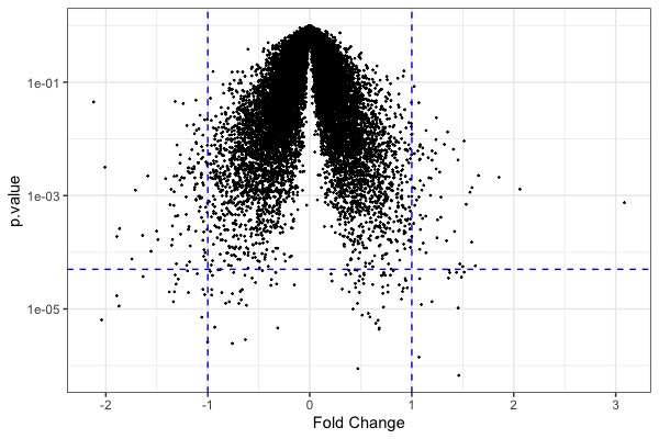
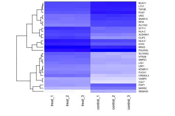
| MA plot | Volcano plot | Heat map |
|---|---|---|
Overview
A genome is the total genetic content of an organism. Driven by breakthroughs such as the decoding of the first human genome and rapid DNA and RNA-sequencing technologies, biomedical sciences are undergoing a rapid & irreversible transformation into a highly data-intensive field, that requires familiarity with concepts in both biological, computational, and statistical sciences.
Genome information is revolutionizing virtually all aspects of life Sciences including basic research, medicine, and agriculture. Meanwhile, use of genomic data requires life scientists to be familiar with concepts and skills in biology, computer science, as well as statistics.
This workshop is designed to introduce computational analysis of genomic data through hands-on computational exercises.
Learning goals
By the end of this workshop students will be able to:
- Manipulate data with R & Rstudio
- Visualize data using R & RStudio
- Analyze microbiome data
Web Links
- Cloud R account (free): https://posit.cloud/; Join the shared work space "NYRaMP-Informatics"
- For your own computer, download the desktop version: https://posit.co/download/rstudio-desktop/
- Textbook: Introduction to R for Biologists
- Download: R datasets
- A reference book: R for Data Science (Wickharm & Grolemund)
Week 1. Aug 5
- Pre-test: visualization, interpretation, and stats. Download file: File:Pre-test.pdf
- Computer/Cloud setup & software download/installation
- R Tutorial 1. Getting started: Basics: interface, packages, variables, objects, functions. Download slides: File:NYRamP bioinformatics 1 slides.pdf
- Session 1 R code: Basic R syntax, working with vectors, and using functions
##### Practice 1 - Together #####

# TASK 1: define a variable that is your name
MyName <- 'Brandon'
print(MyName)
paste('My name is',MyName, sep = ' ')

# TASK 2: output the 3rd and 4th letters in your name using substr function
substr(MyName, start = 3, stop = 4)

# TASK 3: create a vector of the names of all of your Ramp cohort members
roster <- c('Amalya', 'Danny', 'Lorelei', 'Dylan', 'Hadley', 'Brynn', 'Elliot', 'Theo')

# Task 4: check if any of the names have the letters "ic" in them
grepl('an', roster, ignore.case = F)

# Task 5: randomly select 3 names from the roster
sample(roster, size = 3, replace = FALSE)

# TASK 6: combine tasks 4-5
grepl('an', sample(roster, size = 3, replace = F), ignore.case = F)


##### Practice 2 - Independent  #####

library(stringr)

# TASK 1: create a character vector for the DNA nucleotides
Nucleotides <- c('A', 'T', 'C', 'G')

# TASK 2: use the "sample" function on your nuc vector to create a DNA sequence of length 200
DNAseq <- sample(Nucleotides, 200, replace = TRUE)

# collapse the vector into a single string
DNAseq2 <- paste(DNAseq, collapse = '')

# TASK 3: Find out if your sequence contains start codons using the "grepl" function; if output = FALSE, start over
grepl('ATG', DNAseq2, ignore.case = F)

# TASK 4: Find all locations of start codons within your sequence using "str_locate_all" function
str_locate_all(string = DNAseq2, pattern = 'ATG')

# TASK 5: use "substring" function to confirm coordinates are actually "ATG"
'ATG' == substr(DNAseq2, start = 96, stop = 98)

# TASK 6: calculate nucleotide % composition using "str_count" function
str_count(string = DNAseq2, pattern = 'A') / 200 * 100

### alternate more advanced way for tasks 5 and 6 ###

coords <- str_locate_all(string = DNAseq2, pattern = 'ATG')

for (i in 1:nrow(coords[[1]])) {
  start <- coords[[1]][i, 1]
  print('ATG' == substr(DNAseq2, start = start, stop = start+2))
}


for (nuc in Nucleotides) {
  print(paste(nuc,' = ', str_count(string = DNAseq2, pattern = nuc)/nchar(DNAseq2)*100, sep = ''))
}
Week 2. Aug 12
- R Tutorial 2. Data manipulation. Download slides: File:NYRamP bioinformatics 2 slides.pdf
- Session 2 R code:
library(tidyverse)
library(broom)

##### loading a data table #####
df <- read.table('http://wiki.genometracker.org/~weigang/datasets-master/compensation.csv', sep = ',', header = T)
# this loads the data

##### quick look at data #####
dim(df)
nrow(df)
ncol(df)
names(df)
head(df)
glimpse(df)


##### use slice to grab specific rows #####
slice(df, 11:15)
slice_head(df, n=5)
slice_tail(df, n=8)
slice_sample(df, n=20)
slice_max(df, Root, n=3)
slice_min(df, Root, n=3)
slice_min(df, Grazing)

##### arrange function #####
arrange(df, Fruit)
arrange(df, desc(Fruit))
arrange(df, Grazing)
arrange(df, desc(Grazing))


##### filter #####
filter(df, Grazing == 'Grazed')
filter(df, Root < 6.5)
filter(df, Grazing == 'Ungrazed' & Fruit > 50)
filter(df, Fruit > 50 | Root >8)
filter(df,  Grazing == 'Ungrazed' & ( Fruit > 50 | Root >8))

##### piping #####
df %>% #start by calling my dataframe
  select(-Root) %>% # removing the Root data
  filter(Fruit > 50) %>% # keep only fruit with value greater than 50
  arrange(Grazing, Fruit) # arrange first by grazed vs ungrazed, then by fruit size least to greatest

##### computations #####

# operations on an entire column
mean(df$Fruit)
median(df$Root)
sum(df$Fruit)

# operations on individual values in the column
log2(df$Fruit)
df$Fruit / 2

# make a new column by defining and assigning
new_df <- df
new_df$test <- df$Root + df$Fruit

# making a new column based on a computation of data in the df using mutate
new_df <- df %>%
  mutate(log_fruit = log2(Fruit)) %>%
  mutate(combined_mass = Fruit + Root)

##### summary statistics #####
summary(df)

# pipe to get summary by specific variables
df %>%
  filter(Grazing == 'Grazed') %>%
  summary()

# get the stats you want, with grouping
df %>%
  group_by(Grazing) %>%
  summarise(
    mean_fruit = mean(Fruit),
    median_fruit = median(Fruit),
    sd_fruit = sd(Fruit),
    mean_root = mean(Root),
    median_root = median(Root),
    sd_root = sd(Root)
  )


##### rotating a dataframe #####
# add an id so values are in unique rows
df$id <- as.character(1:length(df$Grazing))

# convert to long format
df_long <- df %>% pivot_longer(cols = c(Fruit, Root), values_to = 'value', names_to = 'type')

# you can still group and summarize like you can with the wide format
df_long %>%
  group_by(type, Grazing) %>%
  summarise(
    mean = mean(value)
  )

# convert a long format df to wide
df_wide <- df_long %>% pivot_wider(names_from = type, values_from = value)


##### IRIS DATASET PRACTICE #####
data("iris")

# 1 - Find the dimensions of the dataset
dim(iris)

paste('The iris dataset has',dim(iris)[1],'rows and',dim(iris)[2],'columns.', sep = ' ')

# 2 - List the variables and their data types
glimpse(iris)

# 3 - Summarize the variables
summary(iris)

# 4 - Get the last 10 observations of the dataset
tail(iris, n = 10)
slice_tail(iris, n = 10)

# 5 - Select only the first four columns (remove the “species” column)
select(iris, 1:4)
iris %>% select(1:4)
select(iris, -Species)

# 6 - Filter rows by species, retain only rows from one species (e.g., “setosa”)
filter(iris, Species == 'setosa')
iris %>% filter(Species == 'setosa')

# 7 - Filter rows by a cutoff value (e.g., “Sepal.Length >= 4”)
iris %>% filter(Sepal.Length >= 5)

# 8 - Add a column by taking the log10 of “Sepal.Lengh”
iris %>% mutate(log10_sl = log10(Sepal.Length))

# 9 - What are the medians of the variable “Sepal.Length” for each species?
iris %>%
  group_by(Species) %>%
  summarise(
    median_sl = median(Sepal.Length)
  )

# 10 - Count how many samples for each species
count(iris, Species)
iris %>% count(Species)

# 11 - Convert the table to long format
iris %>%
  pivot_longer(cols = c(Sepal.Length,Sepal.Width,Petal.Length,Petal.Width),
               names_to = 'structure',
               values_to = 'measurement')
Week 3. Aug 19
- R Tutorial 3. Data visualization. Lecture slides: File:NYRamP bioinformatics 3 slides.pdf
- Session 3 R code:
library(tidyverse)
library(broom)
##### compensation dataset viz #####

df <- read.table('http://wiki.genometracker.org/~weigang/datasets-master/compensation.csv', sep = ',', header = T)

# boxplot for root or fruit measurements
df %>%
  ggplot(aes(x = Grazing, y = Root, fill = Grazing)) +
  geom_boxplot() +
  #geom_point()
  geom_jitter(color = 'blue')

# scatter plot with regression line
df %>%
  ggplot(aes(x = Root, y = Fruit, color = Grazing)) +
  geom_point() +
  geom_smooth(method = 'lm')

# bar plot for root or fruit measurement
df %>%
  ggplot(aes(x = Grazing, y = Fruit, fill = Grazing)) +
  geom_bar(stat = 'identity')

# we can do more with a long data format
df_long <- df %>% pivot_longer(cols = c(Fruit, Root), values_to = 'value', names_to = 'type')

# box plot showing root and fruit together
df_long %>%
  ggplot(aes(x = type, y = value, fill = Grazing)) +
  geom_boxplot() +
  geom_jitter() +
  facet_wrap(~type, scales = 'free')


data(iris)
##### compensation dataset hypothesis testing #####
# is there a correlation between root and fruit variables?
cor(df$Root, df$Fruit)

# lets group by to get a better idea
df %>%
  group_by(Grazing) %>%
  summarise(pearson = cor(Root, Fruit))

# is the mean Fruit size the same for grazed and ungrazed?
# t test
t.test(df$Fruit ~ df$Grazing)

# tidy for results in a neat dataframe
res <- tidy(t.test(df$Fruit ~ df$Grazing))

# another way of doing t.test + tidy
t_test <- df %>%
  t.test(Fruit ~ Grazing, data = .) %>%
  tidy()

# linear model - can these variables predict each other?
# can root size predict fruit mass?
lm_simple <- lm(Fruit ~ Root, data = df)
lm_interact <- lm(Fruit ~ Root * Grazing, data = df)

tidy(lm_simple)
tidy(lm_interact)

summary(lm(Fruit ~ Root, data = df))
summary(lm(Fruit ~ Root * Grazing, data = df))
##### iris dataset Viz #####

# simple 1 variable boxplot
iris %>%
  ggplot(aes(x = Species, y = Sepal.Length, fill = Species)) +
  #geom_boxplot() +
  geom_violin() +
  #geom_point()
  geom_jitter()
#geom_bar(stat = 'identity')

# scatter plot for 2 numerical variables
iris %>%
  ggplot(aes(x = Sepal.Length, y = Petal.Length, color = Species)) +
  geom_point() +
  geom_smooth(method = "lm", se = T)


# lets get more information at once!
# convert to long format
df_long <- iris %>%
  pivot_longer(cols = c(Sepal.Length,Sepal.Width,Petal.Length,Petal.Width),
               names_to = 'structure',
               values_to = 'measurement')

df_long %>%
  #filter(structure == 'Sepal.Length') %>%
  ggplot(aes(x = Species, y = measurement, fill = Species)) +
  geom_boxplot() +
  geom_jitter(alpha = 0.5) +
  facet_wrap(~structure, scales = 'free_y')

df_long %>%
  ggplot(aes(x = Species, y = measurement, fill = Species)) +
  geom_bar(stat = 'identity') +
  facet_wrap(~structure)


##### iris dataset hypothesis testing #####
# 1 - is there a correlation between sepal length and sepal width?
cor(iris$Sepal.Length, iris$Sepal.Width)
cor(iris$Sepal.Length, iris$Petal.Length)

# 2 - is there a difference in mean sepal length among the different species?
# anova to compare all three
anova_res <- aov(Sepal.Length ~ Species, data = iris)
# look at results
summary(anova_res)
# post hoc test to see which groups differ
TukeyHSD(anova_res)

# we can do the similar things with t-tests
df <- iris %>%
  filter(Species == 'setosa' | Species == 'virginica')

t.test(Sepal.Length ~ Species, df)$p.value

t_res <- t.test(Sepal.Length ~ Species, data = df)
Demo. Microbiome data analysis
- Mock gene expression data set: File:Sample gene exp dataset.csv
- DNA barcoding dataset, NYC soil microbiome File:Abundance table species.tsv
library(tidyverse)
library(pheatmap)
library(vegan)

setwd('/Users/brandonely/Desktop/informatics_bootcamp/summer_25/')

##### READ DATA #####
df <- read.table('abundance_table_species.tsv', sep = '\t', header = T)

# take a quick look and what we're working with
glimpse(df)
head(df)

##### CLEAN UP DF #####

# lets tackle that tax column and separate it into separate classification levels
df2 <- df %>%
  separate(tax,
           into = c('domain',
                    'kingdom',
                    'phylum',
                    'class',
                    'order',
                    'family',
                    'genus',
                    'species'),
            sep = ';',
            fill = 'warn')

# clean up the genus / species column
df2 <- df2 %>%
  separate(species,into =c('genus2', 'species'),sep = ' ',fill = 'warn') %>%
  select(c(phylum, genus, species, 9:25))

# remove last row of df to avoid downstream issues
df2 <- df2[-nrow(df2), ]


##### PHYLUM LEVEL COMMUNITY COMPOSITION BAR PLOTS #####

# for each phylum, get total read counts per sample
df_phylum <- df2 %>%
  select(-c(genus, species)) %>%  # remove uneeded columns
  group_by(phylum) %>%
  summarise(across(starts_with("barcode"), sum), .groups="drop") # sum counts for each phylum

# convert df to long format
df_phylum <- df_phylum %>%
  pivot_longer(-phylum, names_to="sample", values_to="abundance") # *why the -phylum here?

# calculate relative abundance (normalize)
df_phylum <- df_phylum %>%
  group_by(sample) %>%
  mutate(rel_abundance = abundance / sum(abundance))

# plot
df_phylum %>%
  ggplot(aes(x=sample, y=rel_abundance, fill=phylum)) +
  geom_bar(stat="identity") +
  theme(axis.text.x=element_text(angle=90)) +
  ylab("Relative abundance")

##### ALPHA DIVERSITY (diversity within a single sample) #####

#start prepping data by getting sum of species counts across rows
shannon <- df2 %>%
  select(-c(phylum, genus)) %>%
  group_by(species) %>%
  summarise(across(starts_with("barcode"), sum), .groups="drop")

# convert to a matrix for computations
mat_species <- shannon %>%
  select(-1)
rownames(mat_species) <- shannon$species # set row names as species
mat_species <- as.matrix(mat_species[,-1]) # drop first col since we have it as row names

# calculate relative abundance with operation applied on columns
# this divides every element in a column by the total sum of that column arg1-data, arg2-col or row, arg3-metric, arg4-operation; each column sums to 1
rel_abundance <- sweep(mat_species, 2, colSums(mat_species), '/')

# calculate shannon index with custom function applied on columns
shannon <- apply(rel_abundance, 2, function(p) -sum(p * log(p + 1e-10)))

# prepare final df for platting
shannon_df <- data.frame(sample = names(shannon),
                         shannon = shannon)

# Plot
shannon_df %>%
  ggplot(aes(x = sample, y = shannon, fill = sample)) +
  geom_col() +
  labs(x = "Sample", y = "Shannon Diversity", title = "Alpha Diversity per Sample") +
  theme_minimal() +
  theme(axis.text.x = element_text(angle = 45, hjust = 1), legend.position = 'none')


##### BETA DIVERSITY (Comparing diversity in different samples) #####

# create a dissimilarity matrix between samples using vegdist from vegan package
# transpose b/c we need rows = samples, cols = species
# result is pairwise dissimilarities for all samples
dist_bc <- vegdist(t(rel_abundance), method="bray")

# PCoA analysis
# k=2 dimensions (PC1 and PC2); we're assigning each sample to a space based on 2 coordinates
PCoA <- cmdscale(dist_bc, k=2)

# put coordinates into a df for plotting
PCoA_df <- data.frame(sample = rownames(PCoA),
                      PC1 = PCoA[,1],
                      PC2 = PCoA[,2])

# plot
PCoA_df %>%
  ggplot(aes(x=PC1, y=PC2, color = sample, label=sample)) +
  geom_point(size=3) +
  geom_text(vjust=-0.5) +
  labs(title = 'Beta Diversity') +
  xlab("PCoA1") +
  ylab("PCoA2")
  theme_bw() +
  theme(legend.position = 'none')

# pairwise dissimilarity viz
# we want a normal matrix, not that vegan object
bc_matrix <- as.matrix(dist_bc)

# make the heatmap
pheatmap(bc_matrix,
         clustering_distance_rows = "euclidean",
         clustering_distance_cols = "euclidean",
         main = "Pairwise Bray–Curtis Dissimilarity")

##### GENUS LEVEL COMPARISONS ACROSS SAMPLES HEATMAP #####
# for each genus, get total read counts per sample
df_genus <- df2 %>%
  select(-c(phylum, species)) %>%
  group_by(genus) %>%
  summarise(across(starts_with("barcode"), sum), .groups="drop")

# grab top n genera for plot
top_genera <- df_genus %>%
  mutate(total=rowSums(across(starts_with("barcode")))) %>% # get row sums across all samples
  arrange(desc(total)) %>% # most to least
  slice(1:25) %>% # top n genera
  select(-total) # remove totals column

genus_mat <- as.matrix(top_genera[,-1]) # convert to matrix, drop the genus col
rownames(genus_mat) <- top_genera$genus # make genus column row names of the matrix

pheatmap(genus_mat,
         scale="row", # scale the rows to compare across samples
         clustering_distance_cols="euclidean",
         clustering_method="ward.D2",
         cellwidth = 12,
         cellheight = 8)


