Summer 2018
Rules of Conduct
- No eating, drinking, or loud talking in the lab. Socialize in the lobby only.
- Be respectful to each other, regardless of level of study
- Be on time & responsible. Communicate in advance with the PI if late or absent
Participants
- Dr Oliver Attie, Research Associate
- Brian Sulkow, Research Associate
- Saymon Akther, CUNY Graduate Center, EEB Program
- Lily Li, CUNY Graduate Center, EEB Program
- Mei Wu, Bioinformatics Research Assistant
- Yinheng Li, Informatics Research Assistant
- Christopher Panlasigui, Hunter Biology
- Dr Lia Di, Senior Scientist
- Dr Weigang Qiu, Principal Investigator
- Summer Interns: Muhammad, Pavan, Roman, Benjamin, Andrew, Michelle, Hannah
Journal Club
- a Unix & Perl tutorial
- A short introduction to molecular phylogenetics: http://www.ncbi.nlm.nih.gov/pubmed/12801728
- A review on Borrelia genomics: https://www.ncbi.nlm.nih.gov/pubmed/24704760
- ospC epitope mapping: http://journals.plos.org/plosone/article?id=10.1371/journal.pone.0067445
- Codon usage changes fitness in E.coli: Frumkin et al (2018) "Codon usage of highly expressed genes affects proteome-wide translation efficiency". PNAS
Projects
Borrelia genome evolution (Led by Saymon)
- Goal 1. Estimate time of cross-Atlantic dispersal using core-genome sequences
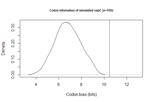
- Goal 2. Investigate codon biases with respect to levels of gene expression. Data file:
* Andrew's BioPython code to calculate CAI
#Opens the fasta file and reads contents into a string (myStr).
myFile = open("B31-cp26.txt","r")
myStr = myFile.read()
myFile.close()

#Imports codon usage module.
from Bio.SeqUtils import CodonUsage as cu

#Takes myStr and processes it into a list of sequences (FastaList).
FastaList = myStr.split(">")
FastaList = FastaList[1:]
IDList = []
EnterList = []
##Separates FastaList into a list of sequence IDs (IDList) and a list of sequences (EnterList).
for seq in FastaList:
    IDList += [seq[:6]]
    EnterList += [seq[6:]]
##Removes enter characters from each sequence in EnterList.
SeqList = []
for seq in EnterList:
    SeqStr = seq.replace("\n", "")
    SeqList += [SeqStr]

#Calculates and presents the CAI value for each sequence using functions from the module.
myObject = cu.CodonAdaptationIndex()
myObject.generate_index("B31-cp26.txt")
for SeqIndex in range(len(SeqList)):
    print (IDList[SeqIndex], '   CAI =', myObject.cai_for_gene(SeqList[SeqIndex]))
Output for cp26:
BB_B01 CAI = 0.7190039074113422
BB_B02 CAI = 0.678404951527374
BB_B03 CAI = 0.6893076488255271
BB_B04 CAI = 0.7250154635421513
BB_B05 CAI = 0.6971190458423587
BB_B06 CAI = 0.67042305582205
BB_B07 CAI = 0.6971020959083346
BB_B09 CAI = 0.6786931743972611
BB_B10 CAI = 0.7224886929887183
BB_B12 CAI = 0.6997502136447451
BB_B13 CAI = 0.7592966148479222
BB_B14 CAI = 0.6959525612884284
BB_B16 CAI = 0.6835709626613392
BB_B17 CAI = 0.6974779110749645
BB_B18 CAI = 0.7052250722958308
BB_B19 CAI = 0.7049049245887261
BB_B22 CAI = 0.6860641572293008
BB_B23 CAI = 0.6915165725213809
BB_B24 CAI = 0.7025276490965267
BB_B25 CAI = 0.7439914547011712
BB_B26 CAI = 0.7255623088410704
BB_B27 CAI = 0.7161378416520467
BB_B28 CAI = 0.7316661839512337
BB_B29 CAI = 0.6919705705489939
- Codon bias by Shannon information: BASH pipeline
- Simulate 100 sequences for each CDS:
cat filename.txt | while read line; do ./codon-info-sim.pl -n 100 BbB31.cutg.GCG "$line".fas > "$line"-sim.fas; done; - Calculate Shannon index for each CDS (simulated & actual)
./codon-info.pl BbB31.cutg.GCG foo.fas
- Simulate 100 sequences for each CDS:
Identification of host species from ticks (Led by Lily [after first-level])
- Goal 1. Protocol optimization for PCR amplification of host DNA from ticks
- Goal 2. Protocol development: library construction for MiSeq
- Goal 3. Development of bioinformatics protocols and sequence database
Pseudomonas Genome-wide Association Studies (GWAS) (Led by Mai & Yinheng, in collaboration with Dr Xavier of MSKCC)
- Goal 1. Association of genes/SNPs with biofilm formation and c-di-GMP levels: Manuscript preparation
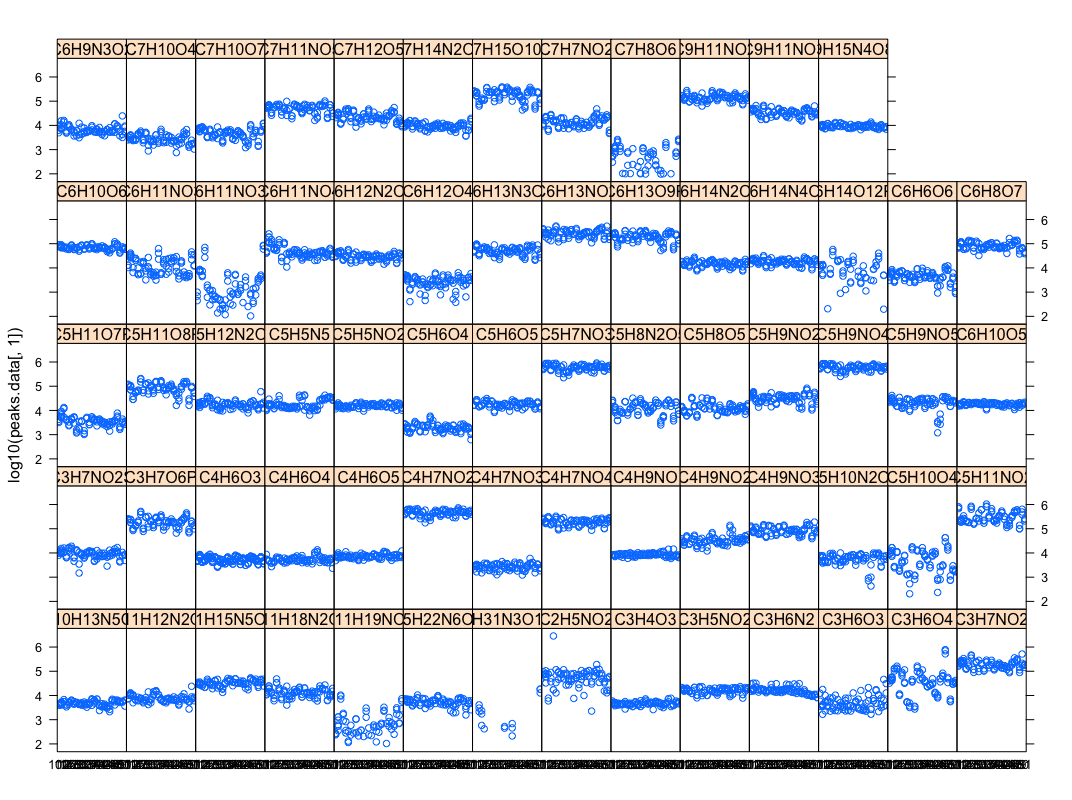
- Goal 2. Association of genome diversity with metabolic diversity
- (Christopher) This script parses excel peak-area file into database & R inputs
#!/usr/bin/perl -w
use strict;
use Data::Dumper;
use Getopt::Std;

my %opts;
my $line_ct = 0;
my (@colnames, @areas, %seen_cmps, %seen_gids);

getopts('dr', \%opts);
while(<>) {
    chomp;
    $line_ct++;
    next unless $line_ct >=4;
    if ($line_ct == 4) {
        @colnames = split "\t", $_;
        for (my $i=5; $i<=$#colnames; $i++) { $seen_gids{$colnames[$i]}++ } # get uniq gids
        next;
    }
    my @data = split "\t", $_;
    $seen_cmps{$data[1]}++; # get unique compound formula
    for (my $i=5; $i<=$#data; $i++) {
        my $area = { 'compound' => $data[1], 'gid' =>$colnames[$i],  'peak_area' => $data[$i]};
        push @areas, $area;
    }
}

if ($opts{d}) { # for database output
    foreach my $cmp (sort keys %seen_cmps) {
        foreach my $gid (sort keys %seen_gids) {
            my @peaks = grep { $_->{compound} eq $cmp && $_->{gid} == $gid } @areas;
            my $peak_str = join ",", map {$_->{peak_area} || "NULL"} @peaks;
            print join "\t", ($gid, $cmp, "{" . $peak_str . "}");
            print "\n";
        }
    }
}

if ($opts{r}) { # for R output
    foreach my $cmp (sort keys %seen_cmps) {
        foreach my $gid (sort keys %seen_gids) {
            my @peaks = grep { $_->{compound} eq $cmp && $_->{gid} == $gid } @areas;
            foreach my $peak (@peaks) {
                next unless $peak->{peak_area};
                print join "\t", ($peak->{peak_area}, $gid, $cmp);
                print "\n";
            }
        }
    }
}
exit;
- (Benjamen) Creates a sample simple force directed network in R using networkD3. Install packages "igraph" and "networkD3".
library(igraph)
library(networkD3)
nodes <- c(rep('x1', 10), rep('x2',10), rep('x3',10), rep('x4',10))
ids <- c(1,1,1,-1,0,-1,0,0,-1,0,0,0,0,0,0,0,0,0,1,-1,0,0,0,0,0,1,-1,-1,0,0,0,0,0,1,-1,0,0,0,0,0)
df <- data.frame(nodes, ids)
df$ids
matrix(df$ids, nrow = 4, ncol = 10, byrow = T)
testmat<-matrix(df$ids, nrow = 4, ncol = 10, byrow = T)
rownames(testmat) <- c("x1", "x2", "x3", "x4")
colnames(testmat) <- c("v1", "v2", "v3", "v4", "v5", "v6", "v7", "v8", "v9", "v10")
testmat.inc <- graph_from_incidence_matrix(testmat)
testmat.edge <- as_edgelist(testmat.inc)
colnames(testmat.edge) <- c("From", "To")
testmat.df <- as.data.frame(testmat.edge)
simpleNetwork(testmat.df, opacity = .8, fontSize = 16)
- (Benjamen) Force-Directed Network Graph Visualization of the iJN746 S Matrix (Only Metabolites in Our Database)
library(igraph)
library(networkD3)

#create a preliminary edgelist from the original matrix. If using the simpleNetwork() function, this
#is the only required step.
stwo <- read.table("Stwo.tsv", header=T)
stwo.inc <- graph_from_incidence_matrix(stwo)
stwo.edge <- as_edgelist(stwo.inc)
colnames(stwo.edge) <- c("from", "to")
stwo.df <- as.data.frame(stwo.edge)

#both the "from" and "to" columns must be given a unique numerical value, as this is the only way
#forceNetwork() will run. To assign numerical values, we index each unique instance of a metabolite
#or reaction in order.

#index "from" column
unique(stwo.edge[,1])
order(unique(stwo.edge[,1]))
from.idx <- data.frame(row.names=unique(stwo.edge[,1]), row.idx=1:82)
stwo.df$from
from.idx[as.character(stwo.df$from),1]
stwo.df$from.idx <- from.idx[as.character(stwo.df$from),1]

#index "to" column
unique(stwo.edge[,2])
order(unique(stwo.edge[,2]))
to.idx <- data.frame(row.names=unique(stwo.edge[,2]), row.idx=1:188)
stwo.df$to
to.idx[as.character(stwo.df$to),1]
stwo.df$to.idx <- to.idx[as.character(stwo.df$to),1]

#add 81 to every value in "to" column and subtract 1 from every value in "from" column. This is so
#the indexing starts from 0, and every indexed variable on the "to" side continues from where "from"
#left off, which, in this case, is variable #82.
stwo.df$to.idx <- stwo.df[,4]+81
stwo.df$from.idx <- stwo.df[,3]-1

#create new data frame with just the "from" and "to" columns.
stwo.new <- data.frame(stwo.df$from.idx, stwo.df$to.idx)
colnames(stwo.new) <- c("from", "to")

#order the edgelist by the to column. The ordered "to" column is then appended to the "from" column,
#and the now disordered "from" column is appended to the "to" column, effectivley mirroring the original
#edgelist. This is done because every variable in the network must show up in the "from" column for
#the forceNetwork() function to work.
stwo.new2 <- stwo.new[order(stwo.new$to),]

#zoom in and out by rolling mouse wheel or double clicking. Click and drag to pan the model.
forceNetwork(Links = links, Nodes = nodes, Source="from", Target = "to", NodeID = "idn", Group = "type.label", linkWidth = 1, linkColour = "green", fontSize = 20, zoom = T, legend = T, Nodesize = 6, opacity = 1, charge = -50, width = 1920, height = 1080)
[http://rpubs.com/benjilev/408463/ Force-Directed Network Graph of iJN746 (Only Metabolites in Our Database)
Machine learning approaches to evolution (Led by Oliver & Brian)
- Goal 1. Implement Hopfield network for optimization of protein structure
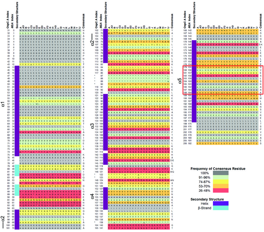
- Goal 2. Neural-net models of OspC. Structural alignment (S2 from Baum et al 2013):
- Goal 3. K-mer-based pipeline for genome classification
Weekly Schedule
- Summer kickoff (June 1, 2018, Friday): Introduction & schedules
- Week 1 (June 4-8):
- Monday: the Unix & Perl Tutorial, Part 1
- Tuesday: Unix Part2. Explore the "iris" data set using R, by following the the Monte Carlo Club Week 1 (1 & 2) and Week 2. Read McKay (2003), Chapters 38 & 39
- Thursday: 1st field day (Caumsett State Park); Participants: John, Muhammad, Pavan, Andrew, Dr Sun, Weigang, with 3 members of Moses team from Suffolk County Vector Control. Got ~110 deer tick nymphs
- Friday: meeting with MSKCC group at 11am; BBQ afterwards
- Week 2 (June 11-15):
- Monday: Lab meeting, projects assigned
- Tuesday: neural net tutorial (by Brian)
- Thursday: 2nd field day (Fire Island National Seashore). Participants: John, Brian, Mei, Muhammad, Pavan, Benjamin, and Weigang. Got ~100 lone-star ticks and 4 deer tick nymphs
- Week 3 (June 18-22):
- Monday: Lab meeting, 1st project reports
- Codon Bias: Theory, Coding, and Data (Andrew, Pavan, Saymon)
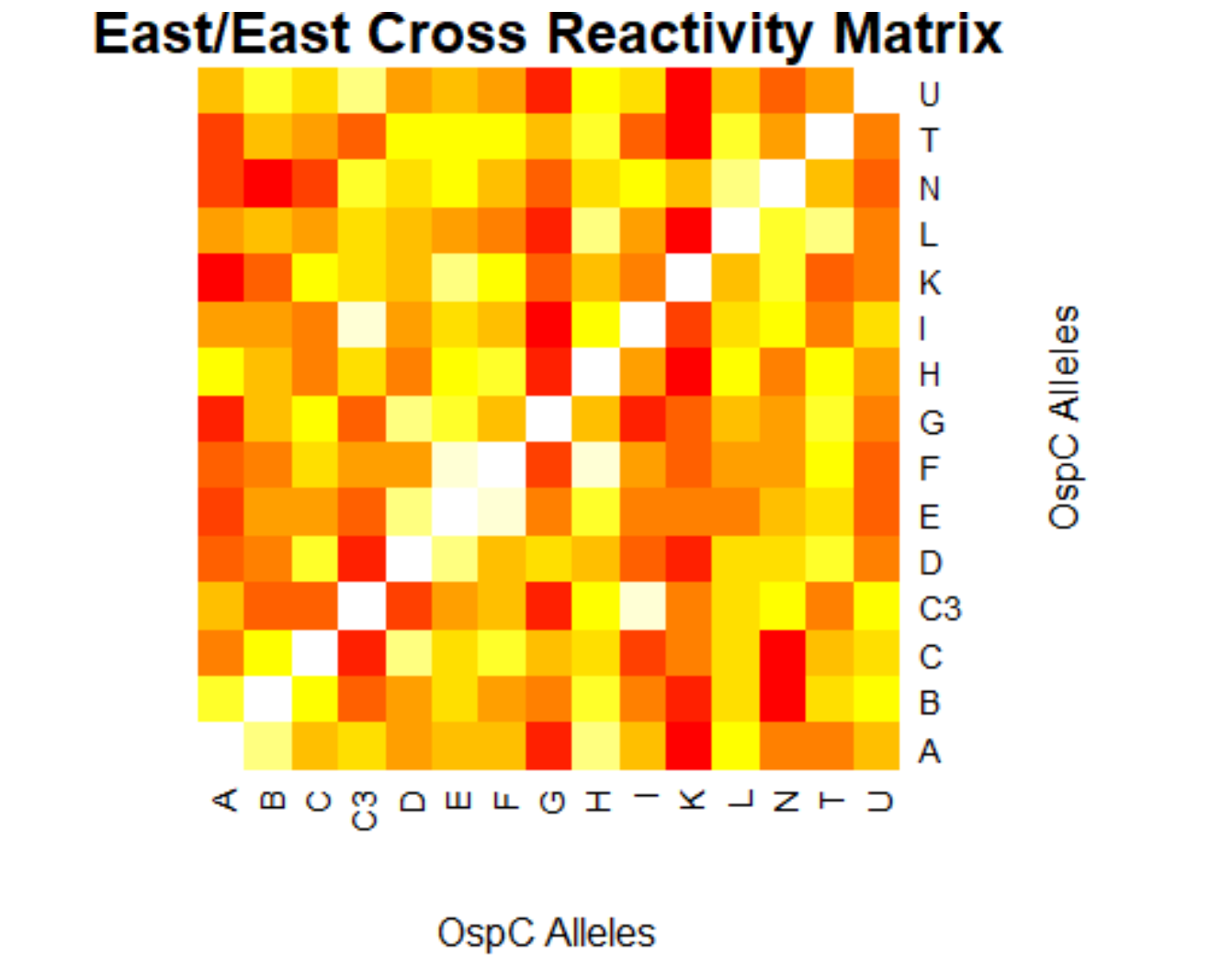
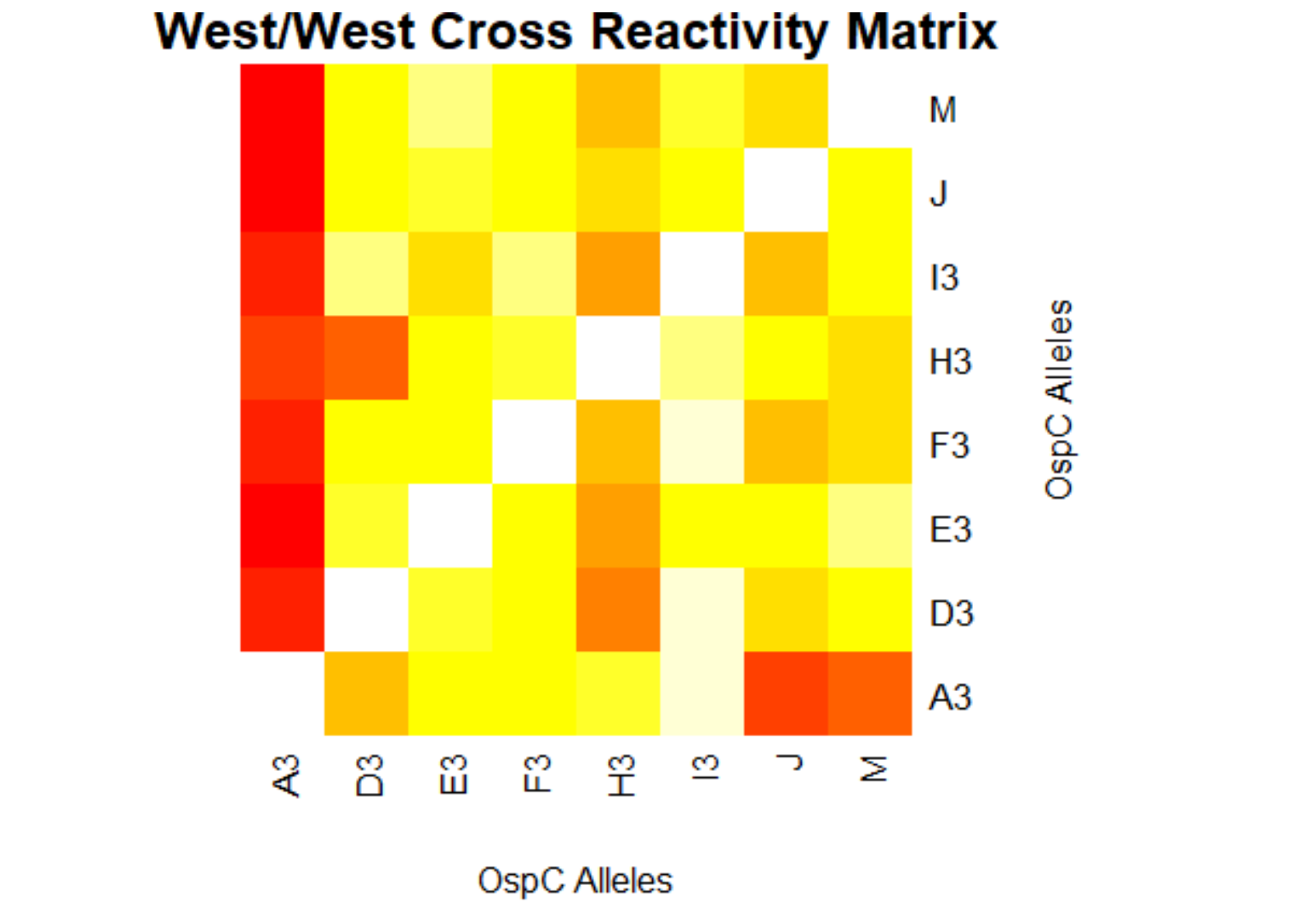
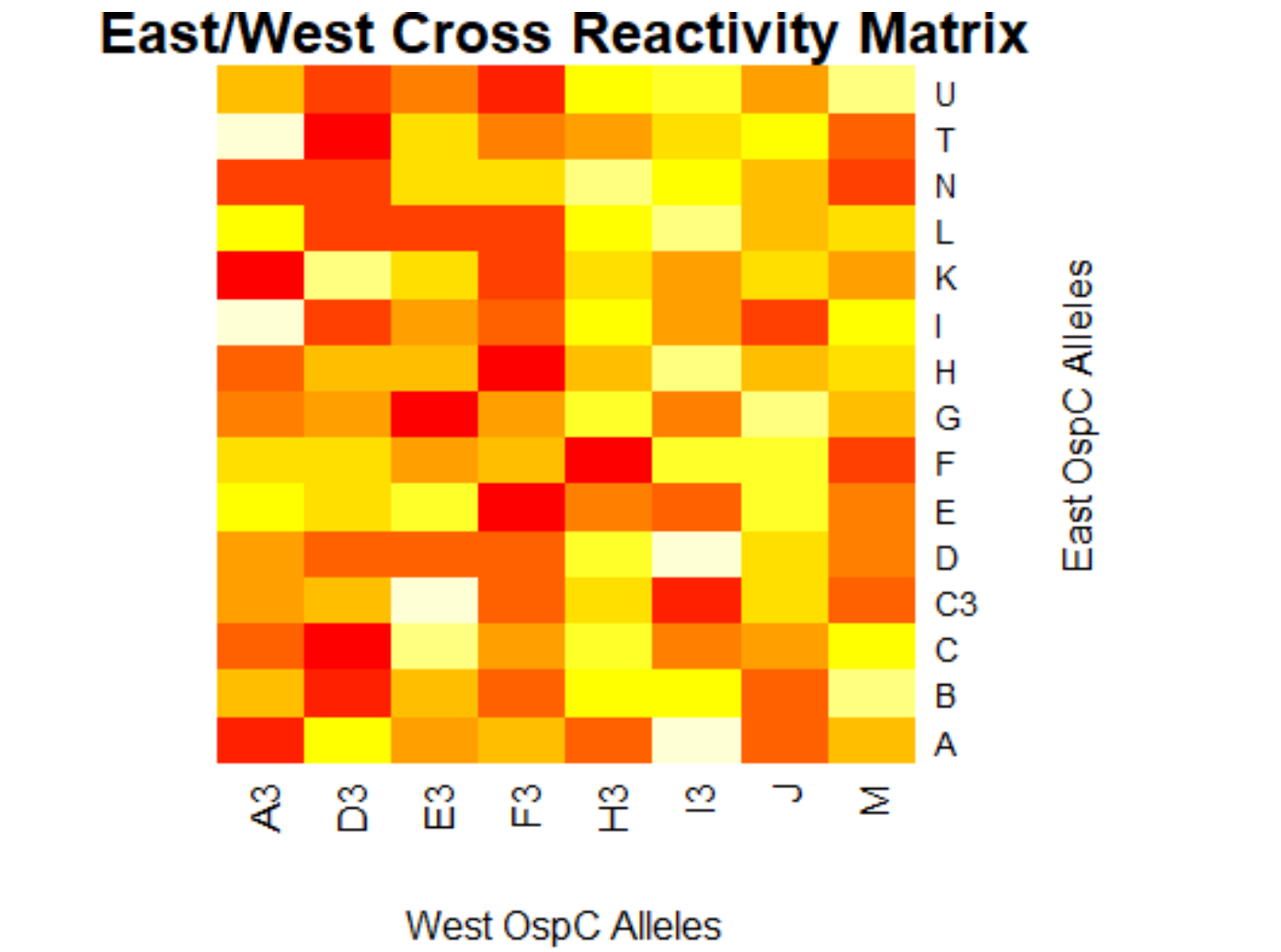
- OspC epitope identification: Serum correlation, sequence correlation, immunity-sequence correction (Muhammad, Roman, Brian)
- Pseudomonas metabolomics: parsing intensity file; theory & parsing SMBL file (Chris & Benjamin)
- Tuesday: working groups
- Wed: working groups
- Thursday: Big Data Workshop
- Friday: working groups
- Monday: Lab meeting, 1st project reports
- Week 4 (June 25-29):
- Monday: Lab meeting
- Tu-Th: work sessions
- Friday: Joint lab meeting with MSKCC/Lab visit
- Week 5 (July 2-6):
- Monday: Lab meeting
- Tuesday/Wed: 4th of July Break
- Thursday & Friday: work sessions
- Week 6 (July 9-13)
- Monday (July 9): E-reports & Wiki posts
- Week 7 (July 16-20)
- Monday (July 16): E-reports * Wiki posts
- Week 8 (July 23-27)
- Monday: lab meeting resumes
Lab notes for Summer HS Interns
- NCI Cloud: Seven Bridges Cloud Platform. Create an user account
- Read documentation & tutorials: Documentation
Notes & Scripts
- (Weigang) A sample R script to parse Table S2 from Baum et al 2013, sera-antigen reactivity measurements
# preliminaries: save as TSV; substitute "\r" if necessary;
# substitute "N/A" to "NA"; remove extra columns
setwd("Downloads/")
x <- read.table("table-s2.txt4", sep="\t", header=T)
View(x)
colnames(x)
which(x[,8]=="A")
x[which(x[,8]=="A"),12]
x[which(x[,8]=="A3"),12]
cor.test(x[which(x[,8]=="A3"),12], x[which(x[,8]=="A"),12], method = "pearson")
x.cor$estimate
levels(x[,8]) # obtain ospC allele types; to be looped through in pairwise
for (i in 1:?) { for (j in ?:?) {cor.test(....)}}
- (Muhammad) Output generates data frame of correlation/p values for 23 different Osp-C allele types in pairwise
setwd("C:/R_OspC")
x <- read.table("Table-S2.txt", sep="\t", header=T)
a<-levels(x[,8])
output = data.frame(i=character(), j=character(), cor = numeric(), p = numeric());
#k <-0;
for(i in 1:22) {
  allele.i <- a[i];
  vect.i <- x[which(x[,8]==allele.i),12];

  for(j in (i+1):23) {
    allele.j <- a[j];
    vect.j <-x[which(x[,8]==allele.j),12];
    cor <- cor.test(vect.i,vect.j, method = "pearson");
    output <- rbind (output, data.frame(i=allele.i, j=allele.j, cor=cor$estimate, p=cor$p.value));
  }
}
 write.table(output, "immune-output.txt", quote = F, sep = "\t")
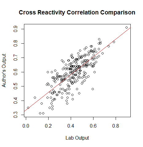
- (Muhammad) Creates a plot for the correlation values of the lab's data and the author's data
#read in the authors cross reactivity correlation matrix
cr<- read.csv("C:/ospc/matricesospc.csv", header=F, sep = ",")
#puts all of the values of cr into corvect
corvect<-c()
for (i in 1:(nrow(cr)-1)) {
  for (j in (i+1):ncol(cr)) {
    corvect[length(corvect)+1]<- cr[i,j]
  }
    }
#merging cross reactivity correlation data and the authors data
df<- data.frame(output, corvect)
#plots the dataframe
plot(output[,3], corvect, main="Cross Reactivity Correlation Comparison", ylab = "Author's Output", xlab="Lab Output")
#gives the liner model, relationship between our data and the authors
b<-lm(corvect~output[,3])
#places the ab line on the plot
abline(b, col=2)
