EEB BootCamp 2020
Jump to navigation
Jump to search
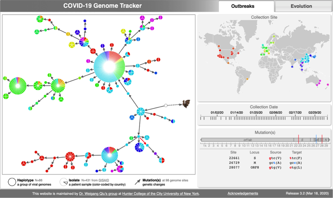
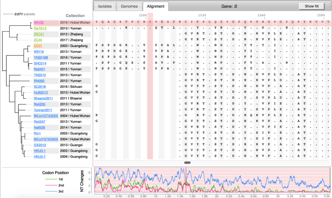
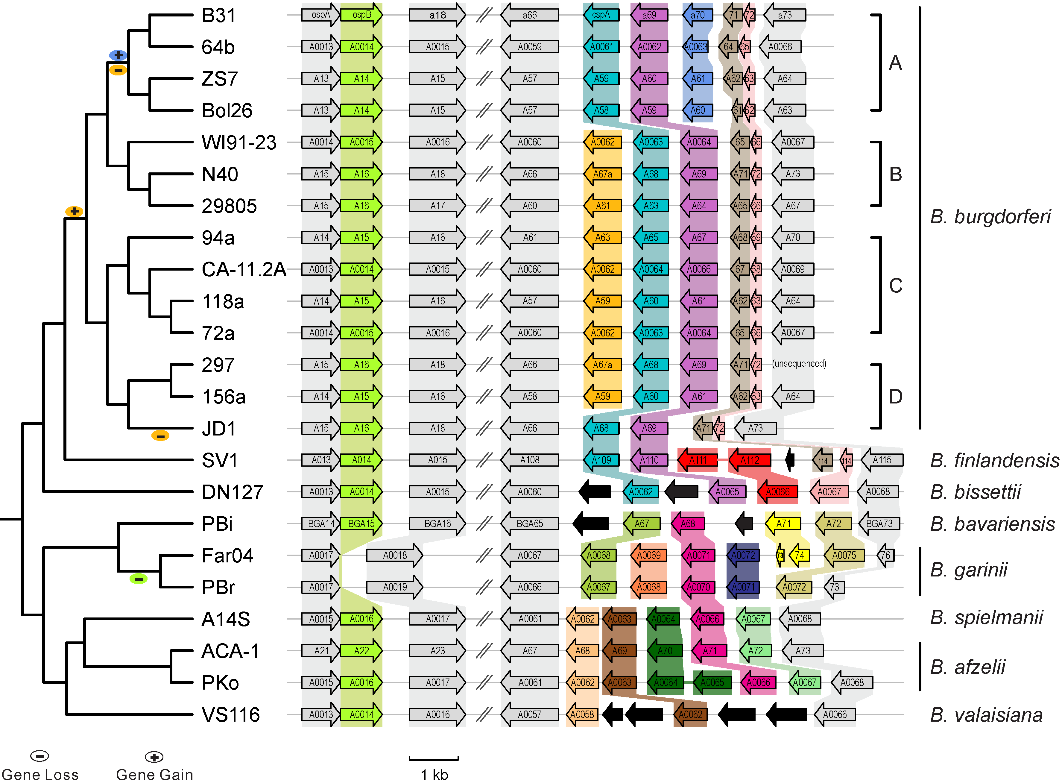
| CoV Genome Tracker | Coronavirus evolutuon | Lyme Disease (Borreliella) |
|---|---|---|
Case studies
Bioinformatics tools for genomic epidemiology
Required for the tutorial
- bcftools: Reading/writing BCF2/VCF/gVCF files and calling/filtering/summarising SNP and short indel sequence variants Installation link
cd bcftools-1.10.2
./configure
make
make install
## You may need sudo permissions to run make install
bcftools --version
# to check the man page
man bcftools
- vcftools: To work with genetic variation data in the form of VCF files Github link Build from Release Tarball
#download version v0.1.16 from second link
cd vcftools-0.1.16
./configure
make
make install
## You may need sudo permissions to run make install

## Alternative: if you have homebrew in your computer
brew install vcftools

vcftools --version
# to check the man page
man vcftools
- Sequence format converter Web tool
- TCS: To infer Haplotype network, TCS.jar file is provided, Required Java. PubMed link
- Web-interactive visualization of Haplotype Network with tcsBU Web tool; Paper
- ggplot (R)
Not required for the tutorial. Recommended
- BpWrapper: command-line tools for manipulation of sequences, alignment, and tree (based on BioPerl). Github Link; Flowchart from publication
- Pairwise genome alignment with MUMMER: Github link
- Samtools: Reading/writing/editing/indexing/viewing SAM/BAM/CRAM format Installation link
CoV genome data set
- N=100 SARS-CoV-2 genomes collected during January, February & March 2020. Data source & acknowledgement GIDAID (Warning: You need to acknowledge GISAID if you reuse the data in any publication)
- Download the folder "bootcamp_august_6th_2020": data file
- unzip the folder
unzip bootcamp_august_6th_2020.zip
- View files
ls -lrt # long list, in reverse timeline

ls cov_data # a folder of 100 CoV2 genomes in FASTA format, pairwise genome alignment sam
            # and indexed sorted bam files generated by bwa (or nucmer) and samtools

# We skipped bwa (or nucmer) and samtools part of the tutorial for time constrain.
#The bash script used to generate these files is available if needed

ls cov_data/*sorted.bam | wc # 100 sorted.bam files correspond to 100 sequence files

less ref.fas # NC_045512 as reference sequence, "q" to quit

less metadata_cov.txt # a tsv file that contains collection dates and geographic information of 100 CoV2 genomes
wc metadata_cov.txt

file TCS.jar # Java application

less bcf-snp-call.sh # a file contain all the bash commands required to call SNPs and generate vcf file of 100 CoV2 genomes
less ploidy.txt # to specify the ploidy=1 during vcf SNP call

less rgb.txt #rgb color code to color the phylogenetic network
- Additional files
#Use this file in part 2 of the tutorial if you couldn't complete SNP call in part 1

less cov_haplotypes.nexus

#Use this file in part 3 of the tutorial to make plot if you couldn't complete SNP call in part 1

less cov_freq_by_continet.txt
Tutorial
- 2-2:30: Introduction on pathogen phylogenomics
- 2:30-2:55: Part 1: Calling SNPs and creating VCF file
## Create alignment pileup and call variants using plodity file(plodity 1), multiallelic, first output is bam then piped to bcf ##

bcftools mpileup -Ou -f ref.fas cov_data/*sorted.bam | bcftools call -mv --ploidy-file ploidy.txt  -Ob -o calls.bcf

## Get Stats, check # of records (SNPs), # of indels, TS/TV ratio
##( expeced more transitions than transversions) #for cov2 should be around more or less 2.5

bcftools stats calls.bcf | less

#remove indels and save into vcf format

bcftools view --exclude-types indels calls.bcf > snps.vcf

## filter sites by allele counts: only keep informative sites

vcftools --vcf snps.vcf --mac 2 --recode --recode-INFO-all --out snps2.vcf

## rename the snp2 recode file

mv snps2.vcf.recode.vcf snps2.vcf

#Get stats, check # of records (informative SNPs) and TS/TV ratio (the ratio will increase)

bcftools stats snps2.vcf | less

## Rename the samples

bcftools query -l snps2.vcf > samples
wc samples
less samples

# make sure you don't have exsiting rename_ids.txt file since we are going to append on the file

if [ -e rename_ids.txt ];then rm rename_ids.txt ; fi
cat  samples | while read line; do basename $line .sorted.bam >> rename_ids.txt ; done;
wc rename_ids.txt

#change the name of the samples

bcftools reheader -s rename_ids.txt snps2.vcf > snps3.vcf
less snps3.vcf

#create fasta file of snps

cat rename_ids.txt | while read line; do echo ">$line"; bcftools query -s "$line" -f '[%TGT]' snps3.vcf; echo; done > cov_haplotypes.fas
grep ">" cov_haplotypes.fas | wc
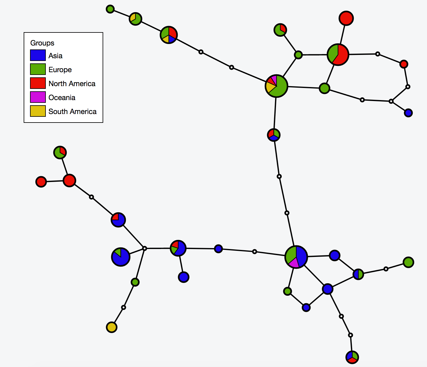
- 2:55-3:10: Part 2: Build and interactive visualize haplotype network with TCS and tcsBU
# Preparing files for haplotype network visualization by parsing the cov metadata
# create file for geographic information

cut -f1,3 metadata_cov.txt | tr '\t' ';' > haplotype.csv
wc haplotype.csv

# Create file to color the network by geography

cut -f3 metadata_cov.txt | sort | uniq > continent.txt
wc continent.txt

paste continent.txt rgb.txt | tr '\t' ';' > groups.csv
less groups.csv

#covert the SNPs fasta file to nexus sequential format
# go to sequence format converter website (find the link in Bioinformatic tools section)

mv result.nexuss cov_haplotypes.nexus
less cov_haplotypes.nexus

#if by any chance you are unable to complete part 1 then please use backup "cov_haplotypes.nexus" file for rest of the steps
# Build haplotype network for the cov dataset

java -jar -Xmx1g TCS.jar

## This part is not command line.
** A java window will pop-up
** Click on "Start New TCS Analysis"
** Fix connection limit at 5 steps
** File -> Select Nexus/Phylip Sequence file -> upload "cov_haplotypes.nexus" file -> Run

# check the output files
ls -lrt

# Interactive visualization of haplotype network with tcsBU
# go to tcsBU website (find the link in Bioinformatic tools section)
** Load graph file -> cov_haplotypes.nexus.graph
** Load group file -> groups.csv
** Load haplotype file -> haplotype.csv
** Show Legend
** Save SVG
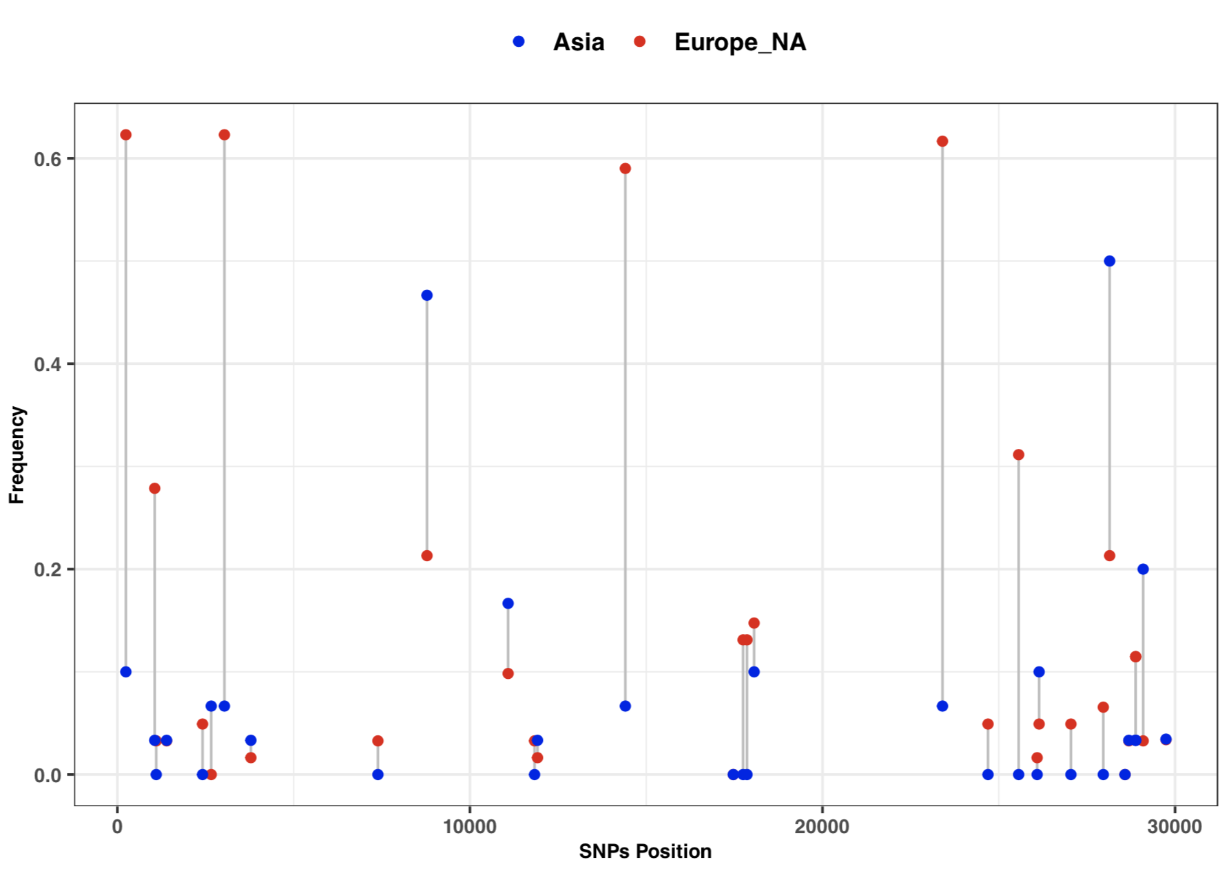
- 3:10-3:25: Part 3: Visualization of SNPs frequency with vcftools and ggplot2
# calculate the SNPs frequency for Europe and North America

grep  -E --  "North America|Europe" metadata_cov.txt | cut -f1 > Europe_NA.ids
wc Europe_NA.ids

bcftools view -S Europe_NA.ids snps3.vcf > Europe_NA.vcf # create Europe and North America subset vcf file
bcftools stats Europe_NA.vcf | less

vcftools --vcf Europe_NA.vcf --freq  --out Europe_NA
less Europe_NA.frq

cut -f2,6 Europe_NA.frq | tail -n +2 | sed $'s/.://'  >  Europe_NA_minor.frq

# calculate the SNPs frequency for Asia

grep  "Asia" metadata_cov.txt | cut -f1 > Asia.ids
wc Asia.ids

bcftools view -S Asia.ids snps3.vcf > Asia.vcf # create Asia subset vcf file
bcftools stats Asia.vcf | less

vcftools --vcf Asia.vcf --freq  --out Asia
less Asia.frq

cut -f2,6 Asia.frq | tail -n +2 | sed $'s/.://' > Asia_minor.frq
less Asia_minor.frq

paste Europe_NA_minor.frq Asia_minor.frq | cut -f1,2,4 > cov_freq_by_continet.txt
less cov_freq_by_continet.txt
wc cov_freq_by_continet.txt

#if by any chance you are unable to complete part 1 then please use backup "cov_freq_by_continet.txt" file for plotting
# SNPs frequency plot by Continent

library(ggplot2)

freq=read.table("cov_freq_by_continet.txt", sep = "\t")
colnames(freq)=c("position", "freq1", "freq2")

ggplot(freq) +
  geom_segment( aes(x=position, xend=position, y=freq1, yend=freq2), color="grey") +
  geom_point( aes(x=position, y=freq1, color='#EA1006'), size=1.5) +
  geom_point( aes(x=position, y=freq2, color='#1A06EA'), size=1.5) +
  scale_colour_manual(name = 'Continent', values =c('#EA1006'='#EA1006','#1A06EA'='#1A06EA'),
                      labels = c('Asia', 'Europe_NA')) +
  theme_bw() + xlab("SNPs Position") + ylab("Frequency") +
  theme(axis.text.y=element_text(size = 8, face = "bold"),
        axis.text.x=element_text(size = 8, face = "bold"),
        axis.title=element_text(size=8,face="bold"),
        legend.title=element_blank(), legend.text=element_text(size=10 , face = "bold"),
        legend.position="top", strip.text.x = element_text(size = 8, face = "bold"))
- 3:25-3:30: Q & A
