Monte Carlo Club
Jump to navigation
Jump to search
March 11, 2017 "Stoplights" (Due 3/18/2017)
- Source: Paul Nahin (2008). "Digital Dice", Problem 18.
- Challenge: How many red lights, on average, will you have to wait for on your journey from a city block m streets and n avenues away from Belfer [with coordinates (1,1)]? (assuming equal probability for red and green lights)
- Note that one has only wait for green light when walking along either the north side of 69 Street or east side of 1st Avenue. On all other intersections, one can walk non-stop without waiting for green light by crossing in the other direction if a red light is on.
- Formulate your solution with the following steps:
- Start from (m+1,n+1) corner and end at (1,1) corner
- The average number of red lights for m=n=0 is zero
- Find the average number of red lights for m=n=1 by simulating the walk 100 times
- Increment m & n by 1 (but keep m=n), until m=n=1000
- Plot average number of red lights by m (or n).
| Submitted Codes |
|---|
import numpy as np
import matplotlib.pyplot as plt
import pandas as pd
from pandas import DataFrame
from random import sample
from itertools import combinations, permutations
from numpy import count_nonzero, array

def red_light(av, st):
    traffic_light = ["red_st", "red_av"]
    total_cross = av + st - 1
    while av != 0 and st != 0:
        if sample(traffic_light, 1)[0] == "red_st":
            av -= 1
        else:
            st -= 1
    rest_cross = av if av != 0 else st
    return(count_nonzero([sample([0, 1], 1) for corss in range(rest_cross)]))

df = DataFrame(0, index=np.arange(10), columns=np.arange(10))

simulation = 1000
for av in df.index:
    for st in df.index:
        df.loc[av, st] = sum(array([[red_light(av, st)] for n in range(simulation)])) / simulation

plt.imshow(df, cmap='hot', interpolation='nearest')
plt.xticks(np.arange(1, 10))
plt.yticks(np.arange(1, 10))
plt.title("Average Numbers Waiting for Red Light")
plt.xlabel("Number of Av")
plt.ylabel("Number of St")
plt.show()

df

# Recursive Function for Each Trial

av = 5
st = 5
traffic_light = ["red_av", "red_st"]
def route(av, st):
    while not av == st == 0:
        if sample(traffic_light, 1)[0] == "red_st":
            if av == 0:
                print("wait at Av. {0} St. {1}".format(av, st))
                return(route(av, st - 1))
            else:
                print("Proceed Av. {0}".format(av - 1))
                return(route(av - 1, st))
        else:
            if st == 0:
                print("Wait at Av. {0} St. {1}".format(av, st))
                return(route(av - 1, st))
            else:
                print("Proceed St. {0}".format(st - 1))
                return(route(av, st - 1))
route(av, st)
# Use recursion
my ($distx, $disty) = @ARGV;
my $num_red = 0; # keep red-light counts
my $xmax = $distx; # needed for text-drawing
print "-" x $xmax, "\n"; # print a starting line
&walk($distx, $disty, \$num_red);
exit;

sub walk {
    my ($x, $y, $ref) = @_;
    my $ct = $$ref;
    my $prob_red;
    if ($x == 1 && $y == 1) { # Arrived at destination
	print "*\n";
	print "-" x $xmax, "\n"; # print the ending line
	print "reached Belfer after waiting for ", $ct, " red lights\n";
    }

    if ($x == 1 && $y > 1) { # Arrived at right-side end
	$prob_red = rand();
	if ($prob_red < 0.5) { # red light, wait
	    $ct++;
	    print "w\n", " " x ($xmax-1);
	} else {
	    print "|\n", " " x ($xmax-1);
	}
	&walk($x, $y-1, \$ct);
    }

    if ($x > 1 && $y == 1) { # Arrived at at bottom
	$prob_red = rand();
	if ($prob_red < 0.5) { # red light, wait
	    $ct++;
	    print "w";
	} else { print "-"}
	&walk($x-1, $y, \$ct, $xmax);
    }

    if ($x > 1 && $y > 1) {
	$prob_red = rand();
	if ($prob_red >= 0.5) { # no red light, move one block right
	    print "-";
	    &walk($x-1, $y, \$ct);
	} else { # red light, move one block down
	    print "|\n", " " x ($xmax-$x);
	    &walk($x, $y-1, \$ct);
	}
    }
}

== March 3, 2017 "PiE" (Due 3/10/2017)==
* Source: Paul Nahin (2008). "Dueling Idiots", Problem 5.
* Challenge: obtain numerical values of Pi and E by simulations
* Simulate pi by [[File:Pi-sim.png|thumbnail]]
# Randomly generate 10,000 pairs of uniformly distributed numbers from 0 and 1 (simulating throwing darts onto the unit square shown at right)
# Count the number of points enclosed within the quarter-circle
# Calculate the pi value from this proportion
* Simulate e by
# Generate N random numbers from 0 to 1
# Divide into N equal-width bins between 0 and 1
# Count the number of bins Z that receive none of the random numbers
# Obtain e ~ N/Z (based on binomial sampling formula)
# Simulate N=1e2, 1e3, and 1e4
{| class="wikitable sortable mw-collapsible"
|- style="background-color:lightsteelblue;"
! scope="col" style="width: 300px;" | Submitted Codes
|- style="background-color:powderblue;"
|
* By Weigang
<syntaxhighlight lang="bash">
# simulate pi:
darts <- sapply(1:1000, function(x) { coords<- runif(2); return(ifelse(coords[1]^2+coords[2]^2 <= 1, 1,0)) })
pi <- 4*mean(darts)

# simulate e
N <- 1e3;
n <- runif(N);
cts <- numeric();
for(i in 1:(N-1)) {
  left <- i/N;
  right <- (i+1)/N;
  cts[i] <- length(which(n>=left & n < right))
}
e <- N/length(which(cts==0))
#Simulate pi
random <- 0; square <- 0;
for (i in 1:1000){
  random[[i]]<- runif(1,0,1)
square[[i]]<- sqrt(1-(random[i])^2)
}
plot(random, square)
areaofqc <- (pi/4)
ranleqc <- length(which(random <=areaofqc))
squleqc <- length(which(square<=areaofqc))

#Simulate e
e <- 0;
for(N in 1:1000) {
  numbers<-runif(N)
bin.size<-1/N
  non.empty<-as.integer(numbers/bin.size)
  z.empt<- N - length(table(non.empty))
  e<-c(e, N/z.empt)
  }
plot(e)
#When you throw a dart at the a unit square dartboard the Probability of hitting the portion of the circle radius with center=(0,0) inside the unit square is  pi/4.  We can say that hitting the 1/4 circle within the unit square with a dart is a bernoulli random variable where p=pi/4. Further, we can say E(bernoulli=hit)=pi/4.
# Imagine you are scoring the game of darts as follows- 1 point if you throw in the 1/4 circle and 0 points if you miss this space.
# If you throw 10000 darts you just did 10000 iid bernoulli trials. By the law of large numbers if we count the number of hits to the 1/4 circle of radius 1 and divide by number of darts thrown we will get something pretty close to E(beroulli) . Multiply that number by 4 and you have an estimate of Pi.

## Generate 10,000 pairs of points in the unit square with uniform distribution

x<-c(runif(1000000, min = 0, max = 1))
y<-c(runif(1000000, min = 0, max = 1))
point<-data.frame(x,y)

plot(point$x,point$y)
point.sub<-subset(point,y<=sqrt(1-x^2))

plot(point.sub$x,point.sub$y)

z<-4*nrow(point.sub)/1000000
z
error<-pi-z
error

## simulating exp
#It's a well that a binomial with large n and tiny p is a good estimate of the poisson random For this estimate lambda=np.  In this case n=10,000 and p=the probability of falling into a particular unit=1/10000.......
 simexp<-function (n) {
a<-c(runif(n,min=0,max=1))
b<-c()

for (i in 1:n) {
  c<-subset(a,(i-1)/n<a & a<=i/n)
  d<-length(c)
  b<-append(b,d)
}
bzero<-subset(b,b==0)
length(bzero)
print(n/length(bzero))
}
simexp(1000)
simexp(10000)
simexp(100000)
#python code
# Simulate pi
simulation = 10000
distances = np.array([pow(uniform(0, 1), 2) + pow(uniform(0, 1), 2) for i in range(simulation)])
pi = count_nonzero(distances < 1) / simulation * 4
pi

# Simulate e
total = 10000
ranges = [[x/total, (x+1)/total] for x in range(total)]
sample_space = [uniform(0, 1) for x in range(total)]
index = []
for i in range(total):
    if any(ranges[i][0] <= point <= ranges[i][1] for point in sample_space):
        index.append(i)
e = total / (total - len(set(index)))
e
|
Feb 24, 2017 "Idiots" (Due 3/3/2017)
- Source: Paul Nahin (2000), "Dueling Idiots". Problem #2: "When Idiots Duel"
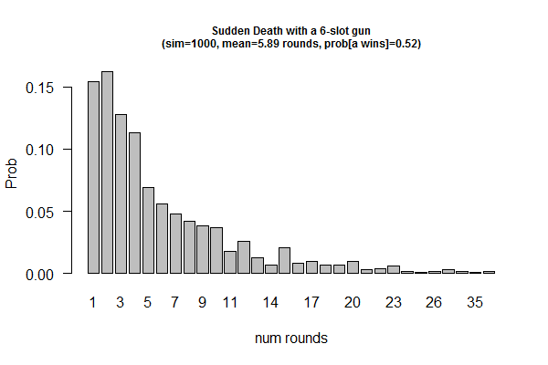
- Game: Idiots A and B decide to duel with a gun in the following way: They will insert a single bullet into the gun's cylinder. The cylinder has a total of 6 slots. Idiot A will spin the cylinder and shoot at B. If the gun doesn't fire, then A will give the gun to B, who will spin the cylinder and then shoot at A. This back-and-forth duel will continue until one fool shoots (and kills) the other.
- Questions: (1) what is the probability that A will win (and B dies); (2) What is the average number of trigger pulls before someone dies?
| Submitted Codes |
|---|
gun <-c(1,0,0,0,0,0)
gun2 <- c(1,0,0,0,0,0)
deadman <-0 ;idiot1win <-0; idiot2win <- 0; nooned <- 0; total <- 0
 while(deadman < 1000){
  idiot1shot <-sample(gun)
  if (length(which(idiot1shot[1] == 1))){
    deadman <- deadman + 1
    idiot1win <- idiot1win + 1
  }else{
      idiot2shot <-sample(gun2)
      if (length(which(idiot2shot[1] == 1))){
        deadman <- deadman +1
        idiot2win <- idiot2win +1
      } else {nooned <- nooned + 1}
  }
  total <- total + 1
  }


deadman
idiot1win
idiot2win
nooned
total

p <- idiot1win/1000
p*100
takes2kill <- deadman/total
takes2kill*100
idiot1shot
idiot2shot
rounds <- sapply(1:1000, function(x) {
  alive <- 1;
  round <- 0;
  while(alive == 1){
    spin <- sample(c(0,0,0,0,0,1));
    round <- round + 1;
    if(spin[1] == 1) { alive <- 0 }
  }
  return(round)
})
prob.a.live <- length(which(rounds %% 2 == 0))
barplot(table(rounds)/1000, xlab="num rounds", ylab="Prob", main = "Sudden Death with a 6-slot gun (sim=1000)", las=1)
|
Feb 17, 2017 "Birthday" (Due 2/24/2017)
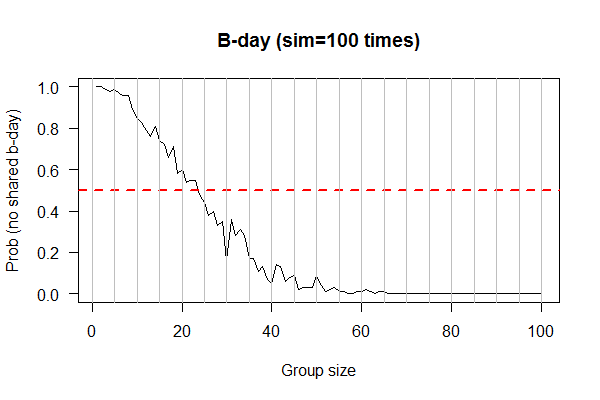
- Problem: What is the probability NONE of the N people in a room sharing a birthday?
- Randomly select N individuals and record their B-days
- Count the B-days NOT shared by ANY two individuals
- Repeat (for each N) 1000 times, and obtain probability by averaging the previous counts (i.e., divided by 1000)
- Vary N from 10 to 100, increment by 10
- Plot probability of no-shared B-Day (Y-axis) versus N (x-axis), with either a stripchart or boxplot, or both
| Submitted Codes |
|---|
N <- 0
samples <- 0;
prob.nodub <-0;
for(j in 10:100){
  counting.no.dups <- 0;
  test <- for(i in 1:1000){
  bdays <- sample(seq(as.Date('1990/01/01'), as.Date('1990/12/31'), by="day"), N, replace=T)
  dups <- duplicated(bdays, incomparables = FALSE)
  ch <-length(which(dups == TRUE))
    if(ch==0){
      counting.no.dups <- counting.no.dups +1
    }
    fine <- (counting.no.dups/1000)
  }
  print(N)
  print(fine)
  N <- N + 1
  samples[[j]] <- N
  prob.nodub[[j]] <- fine
}
plot(samples,prob.nodub, main="Birthday Simulation", xlab = "Sample Size", ylab = "Probability of no Duplicates", las =1)
days <- 1:365;

find.overlap <- function(x) { return(length(which(table(x)>1))) }

output <- sapply(1:100, function(x) { # num of people in the room
  ct.no.overlap <- 0;
  for (k in 1:100) {
    bdays <- sample(days, x, replace = T);
    ct <- find.overlap(bdays);
    if (!ct) { ct.no.overlap <- ct.no.overlap + 1}
  }
  return(ct.no.overlap);
})

plot(1:100, output/100, xlab="Group size", ylab = "Prob (no shared b-day)", las=1, main="B-day (sim=100 times)", type="l")
abline(h=0.5, lwd=2, col=2, lty=2)
abline(v=seq(0, 100, 5), col="gray")
|
Feb 10, 2017 "Dating" (Valentine's Day Special; Due 2/17/2017)
- Source: Paul Nahin (2008), "Digital Dice". Problem #20: "An Optimal Stopping Problem"
- Problem: What is the optimal time point when one should stop dating more people and settle on a mate choice (and live with the decision)
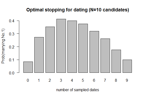
- Your best strategy is to date an initial sample of N individuals, rejecting all, and marry the next one ranked higher than any of your N individuals. The question is what is the optimal number for N.
- The problem could be investigated by simulating a pool of 10 individuals, ranked from 1-10 (most desirable being 1) and then take a sample of N
- You may only date one individual at a time
- You cannot go back to reach previously rejected candidates
- Simulate N from 0 to 9 (zero means marrying the first date, a sample size of zero)
- For each N, obtain the probability of finding the perfect mate (i.e., ranked 1st) by running simulation 1000 times
- Plot barplot of probability versus sample size N.
- Expected answer: N=4
| Submitted Codes |
|---|
pick.candidate <- function(min, array) {
  for (i in 1:length(array)) {
    if (array[i] < min) {
      return(array[i])
    } else {next}
  }
  return(0) # No 1. has been sampled and rejected
}
candidates <- 1:10;
output <- sapply(0:9, function(x) {
  ct <- 0;
  for(k in 1:1000) {
    if (x==0) { # no sample, marry the 1st guy
      sampled <- sample(candidates, 1);
      if (sampled == 1) {ct <- ct+1}
    } else {
      sampled <- sample(candidates, x);
      not.sampled <- candidates[-sampled];
      not.sampled <- sample(not.sampled);
      if (pick.candidate(min =  min(sampled), array = not.sampled) == 1) {ct <- ct+1}
    }
  }
  return(ct);
})
barplot(output/1e3, names.arg = 0:9, xlab = "number of sampled dates", las=1, main = "Optimal stopping for dating (N=10 candidates)", ylab = "Prob(marrying No.1)")
|
Feb 3, 2017 "US Presidents" (Due 2/10/2017)
- Download : 1st column is the order, 2nd column is the name, the 3rd column is the year of inauguration; tab-separated
- Your job is to create an R, Perl, or Python script called “us-presidents”, which will
- Read the table
- Store the original/correct order
- Shuffle/permute the rows and record the new order
- Count the number of matching orders
- Repeat Steps 3-4 for a 1000 times
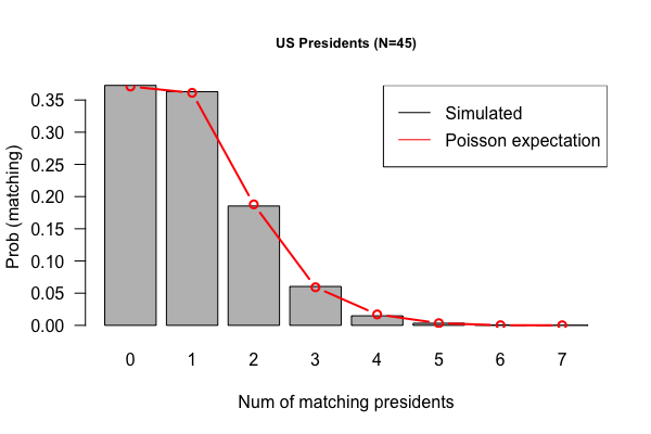
- Plot histogram or barplot (better) to show distribution of matching counts
- Hint: For R, use the sample() function. For Perl, use the rand() function.
| Submitted Codes |
|---|
pres.list <- lapply(1:1000, function(x) pres[sample(nrow(pres)),])
cts <- sapply(pres.list, function(x) {
  ct.match <- 0;
  for (i in 1:45){
    if (pres$order[i] == x[i,1]){
      #cat(as.character(x[i,2]), x[i,1], "\n")  #as.character to avoid the factor info
      ct.match <- ct.match + 1;
      #cat(ct.match)
    }
  }
  ct.match #return
})
barplot(table(cts),xlab = "Number of matches per shuffle", border = "hotpink", col = "pink", ylab = paste("Frequency total of:",length(pres.list)), main = "US Presidents")
import pandas as pd
import numpy as np
from pandas import DataFrame
import matplotlib.pyplot as plt

df = pd.read_table("presidents.txt", names=["num", "name", "presidency"])

name_list = list(df.name)

# create a list to store matches after each shuffle
shuffle_record = []

# create a function in which the first argument is the original dataset; second argument is number of shuffles
def shuffler2(original, n):
    record = []
    for i in range(n):
        num = 0
        each_shuffle = {}
        temp = original.reindex(np.random.permutation(original.index)) # do shuffling for each
        compare = original.num == temp.num
        matched_df = original.ix[compare[compare == True].index]
        for i in matched_df.index:
            each_shuffle[i] = matched_df.name[i]
        shuffle_record.append(each_shuffle)
        try:
            num = compare.value_counts()[1]
        except:
            pass
        record.append(num)
    return(record)
result2 = shuffler2(df, 1000)

plt.hist(result2, color="yellow")
plt.title("Histgram for President Data")
plt.show()
p <- read.table("Presidents.txt", sep="\t", header=F)
colnames(p) <- c("order", "name", "inaug.year")
# Use "sapply" or "lapply" for loops: no need to pre-define a vector to store results
p.sim <- sapply(1:10000, function (x) {
  length(which(sample(p$order) == p$order))
  })
barplot(table(p.sim)/1e4, las=1)
p.exp <- rpois(1e4, 1) # draw 10000 Poisson random deviates
mp <- barplot(table(p.exp)/1e4, las=1, xlab = "Num of matching presidents") # mid-point on x-axis
lines(mp[1:7], table(p.sim)/1e4, type="b", col=2) # add a line (Poisson-expected) to the barplot (simulated)
legend("topright", c("Simulated", "Poisson expectation"), col=1:2, lty=1)
|


