Molecular Evolution (BIOL 375.00/790.64/793.03, Fall 2015)
Instructor: Dr Weigang Qiu, Associate Professor, Department of Biological Sciences
Teaching Assistant: Ms Saymon Akther <saymon.akther@gmail.com>
Room: 926 HN (Seminar Room, North Building)
Hours: Mon. & Thur 4:10-5:25 pm
Office Hours: Belfer Research Building (Google Map) BB-402; Wed 5-7 pm or by appointment
Course Website: http://diverge.hunter.cuny.edu/labwiki/Biol375_2015
Course Description
Molecular evolution is the study of the change of DNA and protein sequences through time. Theories and techniques of molecular evolution are widely used in species classification, biodiversity studies, comparative genomics, and molecular epidemiology. Contents of the course include:
- Population genetics, which is a theoretical framework for understanding mechanisms of sequence evolution through mutation, recombination, gene duplication, genetic drift, and natural selection.
- Molecular systematics, which introduces statistical models of sequence evolution and methods for reconstructing species phylogeny.
- Bioinformatics, which provides hands-on training on data acquisition and the use of software tools for phylogenetic analyses.
This 3-credit course is designed for upper-level biology-major undergraduates. Hunter pre-requisites are BIOL203, and MATH150 or STAT113.
Please note that starting from fall 2015, completing this course no longer counts towards research credits for biology majors.
Textbooks
- (Required) Roderic M. Page and Edward C. Holmes,1998, Molecular Evolution: A phylogenetic Approach, Blackwell Science Ltd.
- (Recommended) Baum & Smith, 2013. Tree Thinking: an Introduction to Phylogenetic Biology, Roberts & Company Publishers, Inc.
Learning Goals
- Be able to describe evolutionary relationships using phylogenetic trees
- Be able to use web-based as well as stand-alone software to infer phylogenetic trees
- Understand mechanisms of DNA sequence evolution
- Understand algorithms for building phylogenetic trees
Links for phylogenetic tools
Exams & Grading
- Attendance (or a note in case of absence) is required. Bonus for active participation in classroom discussions.
- Assignments. All assignments should be handed in as hard copies only. Email submission will not be accepted. Late submissions will receive 10% deduction (of the total grade) per day.
- Three Mid-term Exams (30 pts each)
- Comprehensive Final Exam (50 pts)
Academic Honesty
While students may work in groups and help each other for assignments, duplicated answers in assignments will be flagged and investigated as possible acts of academic dishonesty. To avoid being investigated as such, do NOT copy anyone else's work, or let others copy your work. At the least, rephrase using your own words. Note that the same rule applies regarding the use of textbook and online resources: copied sentences are not acceptable and will be considered plagiarism.
Hunter College regards acts of academic dishonesty (e.g., plagiarism, cheating on examinations, obtaining unfair advantage, and falsification of records and official documents) as serious offenses against the values of intellectual honesty. The College is committed to enforcing the CUNY Policy on Academic Integrity and will pursue cases of academic dishonesty according to the Hunter College Academic Integrity Procedures.
Course Schedule
Part 1. Tree Thinking
- 8/27 (TH). Overview & Introduction. Lecture slides:
| Assignment 1 (10 pts; Due: 8/31, Monday)
|
| Pre-test: Full credits will be given as long as each question is answered with some reasoning. In other words, it will NOT be graded on being right or wrong. It's an assessment tool, to be compared with later test outcomes to show teaching/learning results.
|
- 8/31 (M). 1.1. Introduction (Continued). In-class exercise 1. Tutorial: R & R-Studio (Bring your own computer)
- 9/3 (TH). 2.1. Intro to trees
| Assignment 2 (10 pts; Due: 9/10, Thursday)
|
Watch Origin of Species: Lizards in an Evolutionary Tree. Provide short answer (1-3 sentences) to each of the following three questions.
- What are the two hypotheses explaining the origin of different ecomorphs of lizards on Caribbean Islands?
- What is the expected phylogeny under each hypothesis?
- Which hypothesis is supported by the phylogeny of actual DNA sequences?
|
R exercises
- Install R & R-studio (see "Links for phylogenetic tools" above)
- Open R-studio and install the "ape" package using the "Packages"->"Install" menu, located within the lower right window
- Type in the console window (lower left) the following commands (one at a time, wait for the prompt ">" to appear before proceed to the next command; quit & restart R-studio if stuck):
- library(ape)
- tr = read.tree(text = "(monkey:0.09672,((tarsier:0.18996,lemur:0.14790)0.999:0.09005,(macaque:0.18524,(gibbon:0.10388,(orang-utan:0.09481,(human:0.03391,(gorilla:0.06135,chimpanzee:0.05141):0.01580)0.316:0.05381)1.000:0.03019)0.978:0.05616)0.997:0.05042)0.965:0.09672);")
- plot(tr)
- Export the tree graph using the "Export->Save as PDF or Save as Image" menu in the lower right window
- Exit R studio by typing the command "q()" and type "y" to answer the question for saving the R session
- Copy & paste the tree image into your document to be handed in
|
- 9/7 (M). Labor Day. No class
- 9/10 (TH). 2.2 & 2.3. Tree Distance. In-class exercise 2.
| Assignment 3 (10 pts; Due: 9/17, Th)
|
R exercises
- Download this file & save it in a file folder you could find (e.g., /Users/john/Documents/ for Apple, and C:/Users/john/Documents/ for Windows): . This is an alignment of mitochondrial DNA sequences from primate species, Do not attempt to open or modify it, which may render it un-readable by R. If this happens, delete & re-download.
- Open R-studio and install the "phangorn" package (see Assignment 2 for how to install packages)
- Run the following commands:
- getwd() (this is to show your working directory, from which R-studio could read file)
- setwd("/Users/john/Documents") (to set the working directory to where you saved your mt_primate.txt file)
- library(ape) (this is to load the ape library)
- mt = read.FASTA("mt_primate.txt") (to read the alignment and save it in an object called "mt")
- mt (to show result, copy & paste into your report)
- dist.mt = dist.dna(mt) (to obtain a pair-wise distance matrix)
- dist.raw = dist.dna(mt, model = "raw") (to obtain raw, un-corrected pair-wise sequence differences, in fractions)
- dist.raw * 888 (888 is the length of aligned DNA bases, to show raw counts of base differences; copy & paste into your report)
- tr.mt = bionj(dist.mt) ( to create a tree based on the pairwise distance matrix)
- plot(tr.mt) (to show tree; Export and save tree image)
- library(phangorn)
- tr.mid = midpoint(tr.mt) (this creates a midpoint-rooted tree)
- plot(tr.mid) (Export and save tree image)
- q() (to quit and save your R session, to your working directory)
- Answer the questions:
- Summarize, with your own complete sentences, the key steps you have taken to obtain a tree from sequences.
- Define "monophyly"
- Illustrating with your tree (by labeling ancestral nodes and groups of species), explain why "ape" excluding "human" does not constitute a monophyletic group.
|
- 9/14 (M). No class
- 9/17 (TH). 2.4 & 2.5. Species Tree & Lineage Sorting
- 9/21 (M). 2.5. Consensus Tree & Review. Chapter 2 Slides:File:Part-1-tree-thinking.pdf. In-class Exercise 3:
- 9/24 (TH). 4:10 - 5:10pm Midterm Exam I Bring pencils, erasers, and a calculator
Part 2. Trait Evolution
- 9/28 (M). Traits & trait matrix
| Assignment #4 (5 pts; Due Monday, 10/5)
|
- Download or Copy/Paste the lizard DNA sequences to your own computer and save the file as "lizard.txt"
- Align the DNA sequences using this website and save the aligned DNA file ("Output->Alignment in Fasta format") as "lizard-aligned.txt" (No need to print or submit the above two DNA sequence files; save them for next week's assignment)
- Based on the lizard card, construct a character-state matrix for all lizard species. For each species, list its character state for each of the following two characters (as columns): (1) Geographic origin, and (2) Habitat. Re-watch the video may help this assignment. Hint: use Excel & hand in a printout of your Excel sheet.
|
- 10/1 (TH). Homoplasy & consistency
- 10/5 (M). Parsimony reconstruction (Chapter 5). In-Class Exercise 4:
| Assignment #5 (10 pts; Due 10/15)
|
- Use the DNA alignment from the last assignment to build a tree of Anolis species.
- Set working directory to where you have downloaded the DNA alignment file: e.g., setwd("/Users/ann/Document")
- Load library: library(ape)
- Read alignment: aln.an = read.FASTA("lizard-aligned.txt")
- Calculate pairwise distance matrix: dist.an = dist.dna(aln.an)
- Estimate tree: tr.an = bionj(dist.an)
- Reroot tree: tr.root = root(tr.an, outgroup = "Leiocephalus_barahonensis", resolve.root = T)
- Save tree: write.tree(tr.root, "rerooted.dnd")
- Read re-rooted tree: tr.2 = read.tree("rerooted.dnd")
- Download the phenotype file and save it as "pheno.txt"
- Read phenotype with the command: ph = read.table("pheno.txt", row.names = 1)
- Assign column names: colnames(ph) = c("hab", "geo", "hab_id", "geo_id")
- Plot re-rooted tree: plot(tr.2, x.lim = 1, y.lim = 18, show.tip.label = F)
- Add species names: text(rep(0.2,17), 1:17, tr.2$tip.label, pos=4, font = 3)
- Match species names to tree order: ord = match(tr.2$tip.label, rownames(ph))
- Add a column: text(rep(0.5,17), 1:17, ph[ord,1], pos=4, col = ph[ord,3])
- Add another column: text(rep(0.7,17), 1:17, ph[ord,2], pos=4, col = ph[ord,4])
- Add a heading: text(0.5, 18, "Ecomorph", font = 2, pos=4)
- Add another heading: text(0.7, 18, "Geography", font = 2, pos=4)
- Export & print two copies (in color, preferably)
- On one copy, infer locations (i.e., islands) of all internal nodes using parsimony
- On another copy, infer habitats (i.e., ecomorphs) of all ancestors
- Based on your reconstructed trait evolution, count the number of character-state changes and calculate consistency index for each trait.
- Compare the two consistency indices & explain why the molecular phylogeny supports convergent adaptive evolution to habitats.
|
- 10/8 (TH). Genome & gene structure (Chapter 3)
- 10/12 (M). No Class
- 10/15 (TH). Genome and gene evolution.
- 10/19 (M). Review & Practices. Lecture slides:
- 10/22 (TH). Midterm Exam 2
Part 3. Tree Algorithms
- 10/26 (M). BLAST & Alignments (Chapter 5)
| Assignment #6 (5 pts; Due 11/2)
|
Based on the NCBI Gene Page for cytochrome C (CYCS), answer the following questions:
- What is the molecular function of CYCS?
- Describe its chromosomal location and gene structure (number of introns and exons, length of protein)
- Click the link "HomoloGene" and then in the section "Pairwise alignments generated using BLAST", run BLAST between Human and Mouse protein sequences. Show BLAST report.
- Pick another species and generate a BLAST alignment between the Human and this species. Show BLAST report. Explain the meaning of "Expect" by rephrasing from this page
|
- 10/29 (TH). Maximum parsimony (Chapter 6). In class exercise #6:
- 11/2 (M). Genetic distances (Chapter 6)
| Assignment #7 (10 pts; Due 11/9, Monday)
|
- [Do NOT use computer for this part] Compare these two Ebola VP30 sequences, one from the 2014 outbreak and the other from the 1994 outbreak.
- Calculate the proportion of difference (p) between the two sequences
- Calculate Jukes-Cantor distance (d) between the two sequences (specify unit)
- Count the number of transitions and transversions (arrange in a table, as we did in the class)
- Identify the number of synonymous and nonysynonymous substitutions
- Assuming that the total number of synonymous sites S=174 and the total number of nonsynonymous sites N=690, calculate ds and dn (with Jukes-Cantor correction)
- [Computer Exercise] Calculate & compare genetic distances among the primate mitochondria sequences using R-Studio
- Make sure you have a file "Mt_primate.txt" in your working directory (e.g., "/Users/john/Documents") [Note: Refer back to Assignment #3 if you couldn't locate the file.]
- Load library: library(ape)
- Read alignment: mt = read.FASTA("Mt_primate.txt")
- Calculate raw distance: mt.raw = dist.dna(mt, model = "raw")
- Apply Juke-Cantor (one-parameter model) correction: mt.jc = dist.dna(mt, model = "JC")
- Apply Kimura(two-parameter model, for Ts and Tv) correction: mt.k80 = dist.dna(mt, model = "K80")
- Plot JC distance vs the raw distance: plot(mt.raw, mt.jc, xlab = "uncorrected distance (diff/site)", ylab = "corrected distance (sub/site)", xlim = c(0,0.4), ylim = c(0,0.5), las =1)
- Add a 1:1 line: abline(0,1, col = "red")
- Add K80 distances: points(mt.raw, mt.k80, pch = 3, col = "blue")
- Add a legend: legend(0.05, 0.45, legend = c("JC (1-parameter)", "K80 (2-parameter)"), pch = c(1,3), col = c("black","blue"), bty = "n")
- Export an PDF and print a copy
- Use the graph to explain (1) Why it is necessary to correct for raw distances when comparing sequences from distantly related species; (2) What is the key difference between the K80 and JC models
|
- 11/5 (TH). Distance methods (Chapter 6).
- 11/9 (M). Likelihood methods (Chapter 6)
| Assignment #8 (10 pts; Due 11/16)
|
- Comparison of distance and parsimony trees (review previous assignments for detailed R-Studio instructions)
- In R studio, load the "ape" and "phangnorm" libraries
- Read the "Mt_primate.txt" file, save as "aln"
- Obtain a distance tree:
- Calculate K80 distance matrix, save as "mt.dist"
- Obtain a neighbor-joining tree: tree.nj = NJ(mt.dist)
- Plot a midpoint rooted tree: plot(midpoint(tree.nj))
- Add a scale bar: add.scale.bar()
- Print tree and answer this question: what does the distance represent? What is the unit?
- Obtain a maximum parsimony tree
- Convert object to a different class: aln.phy = as.phyDat(aln)
- Search maximum parsimony tree.mp = optim.parsimony(tree.nj, aln.phy)
- Get tree distance: tree.mp = acctran(tree.mp, aln.phy)
- Plot tree: plot(midpoint(tree.mp))
- Add a scale bar: add.scale.bar()
- Print tree and answer the question: what does the distance represent? What is the unit?
- Compare the two trees and explain the differences in these two methods: Which one uses full sequence information and why?
- Bootstrap analysis
- Read alignment: aln.fas = read.dna("Mt_primate.txt", format = "fasta")
- Create a function for re-rooted distance tree: f = function(x) root(nj(dist.dna(x)), outgroup = c("lemur", "tarsier"), resolve.root = T)
- Calculate a tree: tr = f(aln.fas)
- Perform bootstrap for 100 pseudo-replicates: boot.trees = boot.phylo(tr, aln.fas, f, B=100, rooted =T)
- Plot tree: plot(tr, no.margin = T)
- Add bootstrap values as node labels: nodelabels(boot.trees, bg= "white")
- Explain (1) Does bootstrap test for tree precision or tree accuracy? (2) What does a bootstrap value of 80% mean?
|
- 11/12 (TH). Instructor traveling. No class
- 11/16 (M). Tree-testing & Review (Chapter 6). Lecture slides:
- 11/19 (TH). Midterm Exam 3
Part 4. Population Genetics
- 11/23 (M). Mechanism of molecular evolution: Overview; Analogy with language evolution
- 11/30 (Mon). SNP statistics & Genetic Drift
| Assignment #9 (10 pts; Due 12/7, Monday)
|
|
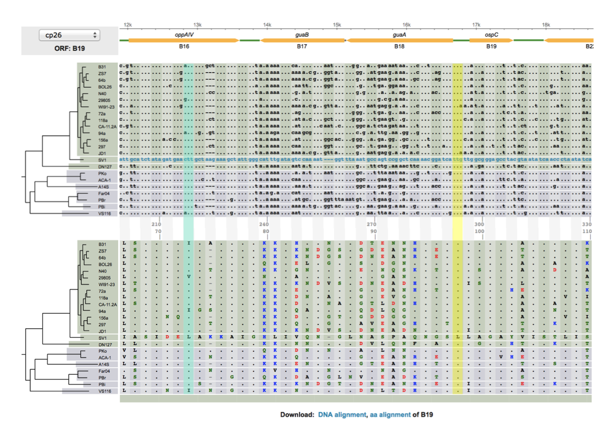
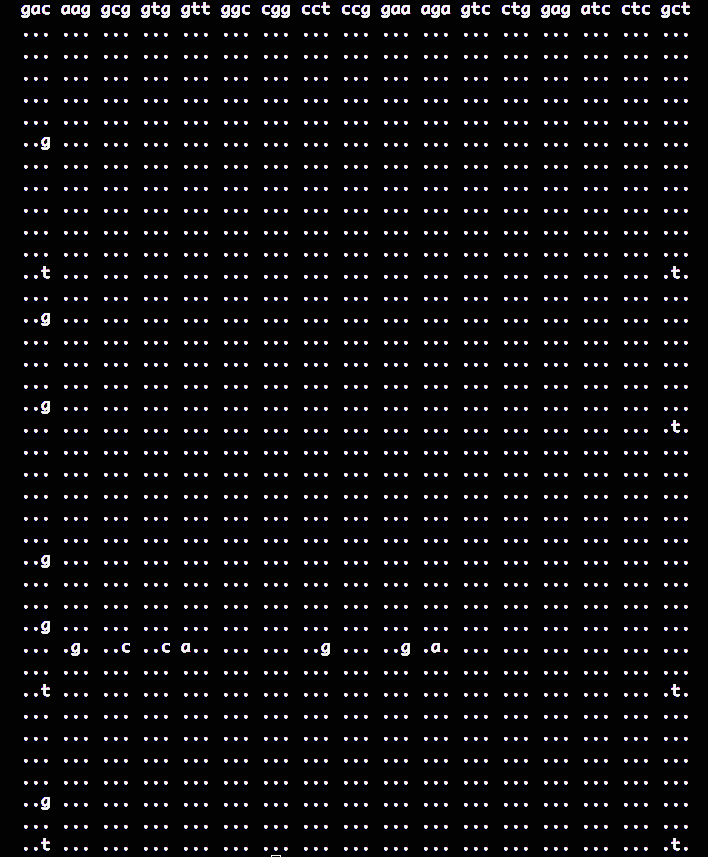
The left figure shows a codon alignment of 38 strains of a bacterium, with an outgroup sequence (which starts with a string of SNPs: "....g...c..ca..", etc), answer the following questions (with the outgroup sequence excluded.) Do not print the figure directly. Hand-copy the sequences to a graph sheet, include only sequences at the two variable codon positions:
- There are two SNP sites. For each SNP, determine whether it is a synonymous or nonsynonymous change (could be both if more than 2 states). You may simply list the codons and their corresponding amino acids, at each aligned codon site.
- Calculate allele frequencies at each SNP site (for 3 SNP states, calculate frequencies of all three separately)
- List all haplotypes using the 2 SNP sites
- Calculate frequencies of all haplotypes
- Using the outgroup sequence, determine the ancestral and derived SNP, codon, and amino-acid states at each codon site. Explain with a tree including the outgroup sequence.
|
- 12/3 (TH). Instructor traveling. No class
- 12/7 (M). Neutral Theory & Molecular Clock
- 12/10 (TH). Tests of Natural Selection. Lecture Slides:
| Assignment # (10 pts; Due 12/14, Monday)
|
Statistical experiments to explore gene-frequency change due to genetic drift:
- With R-studio, make two populations of N=1000 haploid individuals consisting of alleles "A" and "G" at a SNP site:
pop1 = c(rep("A",500), rep("G",500)); pop2 = c(rep("A",100), rep("G",900))
- Count alleles in each population:
table(pop1); table(pop2). Which population is more diverse? Why?
- Define a function to calculate heterozygosity:
hg = function(x) {cts = table(x); total=sum(cts); if (length(cts)==1) {return(0) } else { freq1=cts[1]/total; freq2=cts[2]/total; return(1-(freq1^2+freq2^2)) } }
- Calculate heterozygosity of each population:
hg(pop1); hg(pop2). The results should match your answer to the 2nd question.
- Permute population 1 and take a random sample of 100 individuals:
pop1=sample(pop1); s = sample(pop1, 100); counts=table(s); heterozygosity = hg(s). Is the sample more or less diverse than the original population? Repeat 10 times and report all counts and diversity (e.g., with a table)
- Repeat the above with a smaller sample of 10 individuals
- Repeat with population 2 and a sample of 100 individuals
- Repeat the above with a smaller sample of 10 individuals
- Define "genetic diversity" verbally (+2 pts for giving and using formula for calculating heterozygosity).
- Define "genetic drift". Using results from the above four statistical experiments, discuss the effect of genetic drift to genetic diversity within population. What's the general trend (increase or decrease) of genetic diversity as a result of random sampling of gametes? Is the gain or loss of genetic diversity due to genetic drift more rapid in small or large population (contrasting results with different sample sizes)?
|
- 12/14 (M). Review & Course evaluations.

Answer key to In-Class Exercise 8 Question 2
Review slides:
. Submit your Teacher's Evaluation, using either:
- 12/17 (TH) Comprehensive Final Exam (Regular class hours & Room)
- 12/31 (Wed). Grades Submitted to Registrar Offices (Hunter and Graduate Center)


