Biol425 2013
Jump to navigation
Jump to search
Computational Molecular Biology (BIOL 425/790.49, Spring 2013)
Instructors: Weigang Qiu (Associate Professor of Biology) & Che Martin (Assistant)
Room:1000G HN (10th Floor, North Building, Computer Science Department, Linux Lab FAQ)
Hours: Wednesdays 10:10 am-12:40 pm
Office Hours: Room 839 HN; Wednesdays 5-7pm or by appointment
Contacts: Dr Qiu: weigang@genectr.hunter.cuny.edu, 212-772-5296; Che: cmartin@gc.cuny.edu, 917-684-0864
Attention: Fill out your online Teacher's Evaluation for Spring 2013, available April 15-May16
General Information
Course Description
- Background: Biomedical research is becoming a high-throughput science. As a result, information technology plays an increasingly important role in biomedical discovery. Bioinformatics is a new interdisciplinary field formed between molecular biology and computer science.
- Contents: This course will introduce both bioinformatics theories and practices. Topics include: database searching, sequence alignment, molecular phylogenetics, structure prediction, and microarray analysis. The course is held in a UNIX-based instructional lab specifically configured for bioinformatics applications.
- Problem-based Learning (PBL): For each session, students will work in groups to solve a set of bioinformatics problems. Instructor will serve as the facilitator rather than a lecturer. Evaluation of student performance include both active participation in the classroom work as well as quality of assignments (see #Grading Policy).
- Learning Goals: After competing the course, students should be able to perform most common bioinformatics analysis in a biomedical research setting. Specifically, students will be able to
- Approach biological questions evolutionarily ("Tree-thinking")
- Evaluate and interpret computational results statistically ("Statistical-thinking")
- Formulate informatics questions quantitatively and precisely ("Abstraction")
- Design efficient procedures to solve problems ("Algorithm-thinking")
- Manipulate high-volume textual data using UNIX tools, Perl/BioPerl, R, and Relational Database ("Data Visualization")
- Pre-requisites: This 3-credit course is designed for upper-level undergraduates and graduate students. Prior experiences in the UNIX Operating System and at least one programming language are required. Hunter pre-requisites are CSCI132 (Practical Unix and Perl Programming) and BIOL300 (Biochemistry) or BIOL302 (Molecular Genetics), or permission by the instructor. Warning: This is a programming-based bioinformatics course. Working knowledge of UNIX and Perl is required for successful completion of the course.
- Textbook: Krane & Raymer (2003). Fundamental Concepts of Bioinformatics. Pearson Education, Inc. (ISBN 0-8053-4633-3)
- Academic Honesty: Hunter College regards acts of academic dishonesty (e.g., plagiarism, cheating on examinations, obtaining unfair advantage, and falsification of records and official documents) as serious offenses against the values of intellectual honesty. The College is committed to enforcing the CUNY Policy on Academic Integrity and will pursue cases of academic dishonesty according to the Hunter College Academic Integrity Procedures.
Grading Policy
- Treat assignments as take-home exams. Student performance will be evaluated by weekly assignments and projects. While these are take-home projects and students are allowed to work in groups and answers to some of the questions are provided in the back of the textbook, students are expected to compose the final short answers, computer commands, and code independently. There are virtually an unlimited number of ways to solve a computational problem, as are ways and personal styles to implement an algorithm. Writings and blocks of codes that are virtually exact copies between individual students will be investigated as possible cases of plagiarism (e.g., copies from the Internet, text book, or each other). In such a case, the instructor will hold closed-door exams for involved individuals. Zero credits will be given to ALL involved individuals if the instructor considers there is enough evidence for plagiarism. To avoid being investigated for plagiarism, Do NOT copy from others or let others copy your work.
- Submit assignments in Printed Hard Copies. Email attachments will NOT be accepted. Each assignment will be graded based on timeliness (10%), whether executable or having major errors (50%), algorithm efficiency (10%), and readability in programming styles (30%, see #Assignment Expectations).
- The grading scheme
- Assignments (100 pts): 10 exercises.
- Mid-term (50 pts).
- Final Project (50 pts)
- Classroom performance (50 pts): Active engagement in classroom exercises and discussions
- Attendance (50 pts): 1 unexcused absences = 40; 2 absences = 30; More than 2 = 0.
Assignment Expectations
- Use a programming editor (e.g., vi or emacs) so you could have features like automatic syntax highlighting, indentation, and matching of quotes and parenthesis.
- All PERL code must begin with "use strict; and use warnings;" statements. For each assignment, unless otherwise stated, I would like the full text of the source code. Since you cannot print using the text editor in the lab (even if you are connected from home), you must copy and paste the code into a word processor or a local text editor. If you are using a word processor, change the font to a fixed-width/monospace font. On Windows, this is usually Courier.
- Also, unless otherwise stated, both the input and the output of the program must be submitted as well. This should also be in fixed-width font, and you should label it in such a way so that I know it is the program's input/output. This is so that I know that you've run the program, what data you have used, and what the program produced. If you are working from the lab, one option is to email the code to yourself, change the font, and then print it somewhere else as there is no printer in the lab.
- Recommended Style
- Bad Style
Course Schedule (All Wednesdays)
January 30. Browse Genome & Transcriptome Files with Unix Tools
- Course Overview
- Learning Goal: The power of Unix text filters
- In-Class Exercises:
- You will need these 2 files for the following questions:
/data/biocs/b/bio425/data/GBB.1con, GBB.seq- What is a genome? What does a bacterial genome typically consist of? Explain the following terms: chromosome, plasmids, and contig
- Specify the FASTA file format
- What is the size of the Borrelia burgdorferi (the Lyme disease pathogen) B31 genome in terms of
- Number of replicons: From your home directory, run:
grep -c "^>" ../../bio425/data/GBB.1con [Answer: N=22 replicons]
- Number of genes: From your home directory, run:
grep -c "^>" ../../bio425/data/GBB.seq [Answer: N=1,738 genes]
- Number of bases: First filter out FASTA headers using "grep -v" and then remove newline characters using "tr -d":
grep -v "^>" ../../bio425/data/GBB.1con | tr -d '\n' | wc -m [Answer: N=1,519,856 bases]
- Number of replicons: From your home directory, run:
- Based on the file
/data/biocs/b/bio425/data/ge-breast-cancer-cell-lines.dat, answer the following questions:- What is a transcriptome?
- How many unique genes are represented in this chip?
cut -f1 ../../bio425/data/ge-breast-cancer-cell-lines.dat | grep -vc "^Description" [Answer: N=18,900 genes]
- How many cell lines in the file?
grep "^Description" ../../bio425/data/ge-breast-cancer-cell-lines.dat| cut -f2- | wc -w [Answer: N=59 cells]
- Extract gene expression values at 3 breast cancer clinical markers: ERBB2, ESR1, and PGR
grep -wP "ERBB2|ESR1|PGR" ../../bio425/data/ge-breast-cancer-cell-lines.dat [You should see 3 rows of gene expression values]
| Assignment #1 (Final Version; Q4 file name corrected) |
|---|
Unix Text Filters
|
| Read Chapter 1 |
February 6. Central Dogma with PERL (Part 1)
- Learning goals:
- DNA Replication and Transcription
- String manipulations using BASH & PERL
- In-Class Exercises:
- Find out base composition (%A, %T, %C, and %G) of a DNA sequence
- In the folder
/data/biocs/b/bio425/data/GBB.1con-splitted, the whole B. burgdorferi genome has been splitted into files each of which containing a single replicon. Write a short BASH script to count how many bases in each replicon.for f in ../../bio425/data/GBB.1con-splitted/*.fas; do echo -ne "$f\t"; grep -v "^>" $f | tr -d "\n" | wc -m; done
- Write a PERL script to count GC% given a FASTA sequence.
Script posted at /data/biocs/b/bio425/scripts/gc-counter.pl
- Run the GC-counter for each replicon using a BASH loop.
for f in ../../bio425/data/GBB.1con-splitted/*.fas; do perl /data/biocs/b/bio425/scripts/gc-counter.pl $f; done
- In the folder
- Central Dogma
- Illustrate the Central Dogma using lines representing DNA/RNA/Protein. Indicate directionality of all parts.
DNA replication, Transcription & Translation: all 5' to 3'
- Define cDNA. What are some of the common uses of cDNA?
Identify alternative-splicing variants (isoforms); Quantify gene expression levels (RNA-SEQ)
- Illustrate the Central Dogma using lines representing DNA/RNA/Protein. Indicate directionality of all parts.
- DNA replication
- What is the implied directionality of a DNA sequence if none is specified?
5' to 3'
- What is the complement strand of this DNA sequence
gatactaatgaagtatin 5' to 3' direction?atacttcattagtatc
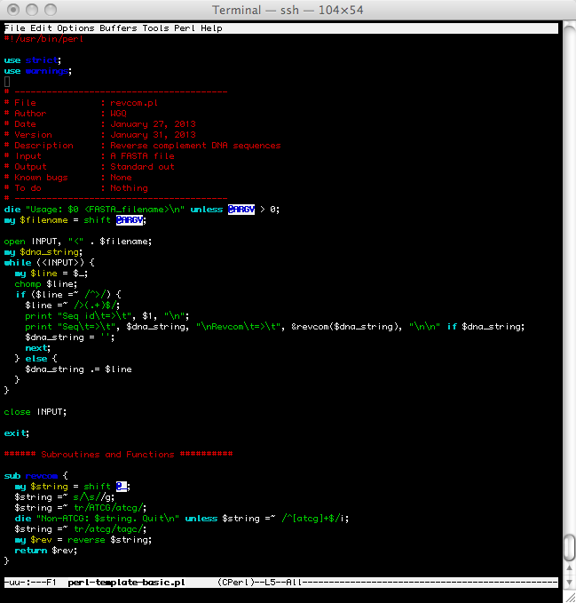
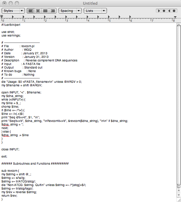
- Write a PERL script to output the complementary strand of the ospC gene
/data/biocs/b/bio425/data/ospC.seqin 5' to 3' direction. Save the result in a FASTA fileospC.revcom.fasScript posted at /data/biocs/b/bio425/scripts/revcom.pl
- What is the implied directionality of a DNA sequence if none is specified?
| Assignment #2 (Final) |
|---|
|
February 13. Central Dogma with PERL (Part 2)
- Learning goals: DNA translation & ORF Identification
- In-Class Exercises:
- Six-frame translation
- Define ORF and reading frame. How many possible reading frames are there for a given sequence?
ORF: Hypothetical, computer-predicted protein-coding sequences. An ORF needs experimental data (e.g., mRNA) to be verified as a true gene. There are six possible reading frames for a given DNA sequence: three (+1, +2, +3) on one strand and another three (-1, -2, -3) on the reverse-complement strand.
- How does a cell normally choose only one reading frame out of other possibilities for any given parts of a genome?
In a prokaryotic cell, transcription factors (TFs) bind to a particular sequence (called "promoters") at the 5'-upstream of an ORF. TFs recruits RNA polymerase to initiative the transcription of a gene. After the transcription, ribosomes bind to another particular 5'-upstream sequence (SD sequence, normally "AGGAG") to start the translation of a protein.
- Using a DNA genetic code table to manually translate the following sequence in all possible reading frames:
gatactaatgaagtat. Which reading frame do you think is the most likely one?+1: DTNEV; +2: ILMKY; +3:Y**S; -1:ILH*Y; -2:YFISI; -3:TSLV. Frames +3 and -1 could be eliminated.
- Define ORF and reading frame. How many possible reading frames are there for a given sequence?
- ORF identification in a bacterial genome
- Pick a plasmid sequence from
/data/biocs/b/bio425/data/GBB.1con-splittedRun ls -lh ../../bio425/data/GBB.1con-splitted/ and choose a small plasmid file, e.g., Borrelia_burgdorferi_4041_cp9_plasmid_C.fas
- Identify ORFs on the plasmid by running the program
/data/biocs/b/bio425/bin/long-orfs/data/biocs/b/bio425/bin/long-orfs /data/biocs/b/bio425/data/GBB.1con-splitted/Borrelia_burgdorferi_4041_cp9_plasmid_C.fas cp9.coord
- Extract ORF sequences using the program
/data/biocs/b/bio425/bin/extract/data/biocs/b/bio425/bin/extract /data/biocs/b/bio425/data/GBB.1con-splitted/Borrelia_burgdorferi_4041_cp9_plasmid_C.fas cp9.coord
- Pick a plasmid sequence from
| Assignment #3 (Final Version) |
|---|
|
February 20 (No Class)
- Monday Schedule
February 27. Genomics with BioPerl (Part 1)
- Learning goals: Introduction to Objects
- In-Class Exercises:
- Construct a sequence object with a hash
- Select and write down at least five features (e.g., strain, gene) associated with a DNA sequence based on this GenBank record. Include a sequence label and the sequence itself as two of the features.
- Write a PERL program named "seq_object.pl", which captures these five features with a hash by using feature names as keys and features as values. Example:
my %seq_obj=("strain"=>"SD91, "gene"=>"ospC");Print the hash with Data::Dumper.my $seq_hash=("id"=>"SD1_ospC", "seq"=>"tgtaataattcaggaaaaga", "organism"=>"Borrelia burgdorferi", "strain"=>"SD1", "gene"=>"ospC"); print Dumper(\%seq_hash) - Create a scalar variable called "$ref_seq_obj", which is a reference to the hash %seq_obj. Print the hash reference with Data::Dumper.
my $ref_seq_obj=\%seq_obj; print Dumper($ref_seq_obj)
- Name some of the differences between a sequence and a sequence object.
Sequence refers to a string of nucleotides or amino acids. A sequence is usually represented by a string variable. A sequence object includes biological features associated with a sequence besides the sequence itself. A sequence object is commonly represented by a hash reference in Perl.
- Construct a sequence object with Bio::Seq
- Modify your program by calling the Bioperl Bio::Seq module:
use lib '/data/biocs/b/bio425/bioperl-live'; use Bio::Seq;
- Convert your hash-based sequence object into a Bio::Seq object:
my $seqobj = Bio::Seq->new( -display_id => "SD1_ospC", -seq =>"tgtaataattcaggaaaaga" );
- Print the Bio::Seq object with Data::Dumper
print Dumper($seqobj);
- Modify your program by calling the Bioperl Bio::Seq module:
- Apply Bio::Seq methods
- Find the names of methods for the following operations on the Bio::Seq object: reverse complement, length, id, seq, translate, sub-sequence by running
perldoc /data/biocs/b/bio425/bioperl-live/Bio/Seq.pm
- Add the above methods into your script & print all results
my $seq_rev=$seqobj->revcom()->seq(); my $eq_length=$seqobj->length(); my $seq_id=$seqobj->display_id(); my $seq_string=$seq_obj->seq(); my $seq_translate=$seqobj->translate()->seq(); my $subseq = $seqobj->subseq(1,10)
- Find the names of methods for the following operations on the Bio::Seq object: reverse complement, length, id, seq, translate, sub-sequence by running
- Discussion Questions
- What is Object-oriented Programming?
- What is an Object and what is a Method?
A Perl object is a "blessed" (strictly defined) reference to a hash. A method is a subroutine or function associated with an object. An object and its associated methods together make a class (e.g., the Bio::Seq class).
- What are the advantages and disadvantages of Object-Oriented programming in comparison with traditional programming based on subroutines and functions?
Advantages: Simpler and more readable code. Easier maintenance. Disadvantages: Code dependent on installation of external libraries (e.g., BioPerl). An extra layer of abstraction, e.g., the concept of objects and methods.
| Assignment #4 (Final version) |
|---|
|
March 6: Genomics with BioPerl (Part 2)
- Learning goal: File I/O with BioPerl
- In-Class Exercises:
- Read a FASTA file with Bio::SeqIO
- Find out how to read a FASTA file using Bio::SeqIO by running
perldoc /data/biocs/b/bio425/bioperl-live/Bio/SeqIO.pm
- Write a PERL script
fasta-io.pl, which uses Bio::SeqIO to read a multi-FASTA file (input) and print the name and length of each sequence (output). Test your script on this file../../bio425/data/Borrelia_osp.dna.fasta
- Find out how to read a FASTA file using Bio::SeqIO by running
- Output a FASTA file with Bio::SeqIO
- Find out how to output a FASTA file using Bio::SeqIO by (again) running
perldoc /data/biocs/b/bio425/bioperl-live/Bio/SeqIO.pm
- Modify the PERL script
fasta-io.plto read a multi-FASTA file (input) and print a translation of each sequence (output). Test your script on this file../../bio425/data/Borrelia_osp.dna.fasta
- Find out how to output a FASTA file using Bio::SeqIO by (again) running
- Start working on assignment 5 (see below) if you have time.
| Assignment #5 (Final Version) |
|---|
|
March 13: Mid-Term Review
- In-class Exercise: Write a BASH script named as "get-long-orfs.bash" to output long ORFs and their translated protein sequences given a genome sequence. Your script will combine commands and scripts you have previously composed into a single-command utility.
- Input file: Locate whole plasmid sequences in the "/data/biocs/b/bio425/data/GBB.1con-splitted/" folder:
- Group 1: use "Borrelia_burgdorferi_4075_lp54_plasmid_A.fas"
- Group 2: use "Borrelia_burgdorferi_4091_cp26_plasmid_B.fas"
- Group 3: use "Borrelia_burgdorferi_4041_cp9_plasmid_C.fas"
- Group 4: use "Borrelia_burgdorferi_4076_lp17_plasmid_D.fas"
- Group 5: use "Borrelia_burgdorferi_4005_lp25_plasmid_E.fas"
- Output files: two files (2 bonus points if your output file names are generated dynamically, not hard-coded)
- "plasmid_X.nuc": ORF sequences in FASTA
- "plasmid_X.pep": Protein sequences in FASTA
- Input file: Locate whole plasmid sequences in the "/data/biocs/b/bio425/data/GBB.1con-splitted/" folder:
filename=$1; base=$(basename $filename ".fas"); coordfile=$base.coord; nucfile=$base.nuc; pepfile=$base.pep; /data/biocs/b/bio425/bin/long-orfs -A ATG -g 200 $filename $coordfile; perl extract.pl $filename $coordfile > $nucfile; perl extract-bioperl-version.pl $filename $coordfile > $pepfile
- Sample Questions:
- Define elements of a prokaryotic gene: ORF, promoter, RBS-binding sites
- Construct a single "for" loop to translate a sequence in six frames
- Print the reverse-complement sequence given a Bio::Seq object
- Mid-term will cover the following contents (Review all in-class exercises and assignments)
- Biology: genome, transcriptome, 6-frame translation, gene structure
- Linux file system & text tools: ls [-lart]; less; grep [-ivcwP]; cat; cut [-fd]; head; tail; bash script (for loop); tr; wc [-lwm]
- Gene-finding using GLIMMER: long-orfs, extract
- Basic Perl: file I/O; loops (for; foreach; while); regex; using hash for counts and translation
- Object-oriented BioPerl: the use Bio::SeqIO & Bio::Seq
March 20. Midterm Practicum
March 27 (No Class)
See assignments above
April 3: Transcriptome with R (Part 1)
- Learning goal: Introduction to R
- R resources
- Forget about Excel! Instead, use R for statistical analysis and visualization of large data sets.
- Download and install R to your own computer from: R website
- Download and install R studio to your own computer from: R Studio website
- A nice tutorial: SimpleR
- In-Class Exercises: Part 1.
- Set a working directory
- Using a Linux terminal, make a directory called
R-work - Start R-Studio (Note: This link works only if you use computers in the 1000G lab. Install and use your own R Studio for homework assignments)
- Find working directory with
getwd() - Change working directory with
setwd("~/R-work")
- Using a Linux terminal, make a directory called
- The basic R data structure: Vector
- Construct a character vector with
c.vect=c("red", "blue", "green", "orange", "yellow", "cyan") - Construct a numerical vector with
n.vect=c(2, 3, 6, 10, 1, 0, 1, 1, 10, 30) - Construct vectors using functions
n.seq1=1:20n.seq2=seq(from=1, to=20, by=2)n.rep1=rep(1:4, times=2)n.rep2=rep(1:4, times=2, each=2)
- Use built-in help of R functions:
?seqorhelp(seq) - Find out data class using the class function:
class(c.vect)
- Construct a character vector with
- Access vector elements
- A single value:
n.vect[2] - A subset:
n.vect[3:6] - An arbitrary subset:
n.vect[c(3,7)] - Exclusion:
n.vect[-8] - Conditional:
n.vect[n.vect>5]
- A single value:
- Apply functions
- Length:
length(n.vect) - Range:
range(n.vect); min(n.vect); max(n.vect) - Descriptive statistics:
sum(n.vect); var(n.vect); sd(n.vect) - Sort:
order(n.vect). How would you get an ordered vector of n.vect? [Hint: use?orderto find the return values] - Arithmetics:
n.vect +10; n.vect *10; n.vect / 10
- Length:
- Quit an R session
- Click on the "History" tab to review all your commands
- Save your commands into a file by opening a new "R Script" and save it as
vector.R - Save all your data to a default file .RData and all your commands to a default file ".Rhistory" with
save.image() - Quit R-Studio with
q()
- In-Class Exercises: Part 2
- Start a new R studio session and set working directory to
~/R-work - Generate a vector of 100 normal deviates using
x.ran=rnorm(100) - Visualize the data distribution using
hist(x.ran) - Explore help file using
?help; example(hist) - How to break into smaller bins? How to add color? How to change x- and y-axis labels? Change the main title?
- Test if the data points are normally distributed.[Hints: use qqnorm() and qqline()]
- Save a copy of your plot using "Export"->"Save Plot as PDF"
- In-Class Exercises: Part 3
- Using a Linux terminal, make a copy of breast-cancer transcriptome file
/data/biocs/b/bio425/data/ge.datin your R working directory - Start a new R studio session and set working directory to
~/R-work - Read the transcriptome file using
ge=read.table("ge.dat", header=T, row.names=1, sep="\t")- What is the data class of
ge? - Access data frame. What do the following commands return?
ge[1,]; ge[1:5,]; ge[,1]; ge[,1:5]; ge[1:5, 1:5] - Apply functions:
head(ge); tail(ge); dim(ge)
- What is the data class of
- Save a copy of an object:
ge.df=ge. - Transform the transcriptome into a numerical matrix for subsequent operations:
ge=as.matrix(ge) - Test if the expression values are normally distributed.
- Save and quit the R session
| Assignment #6 (Final Version) |
|---|
|
April 10: Transcriptome with R (Part 2)
- Learning goal: Classification of breast-cancer subtypes
- In-Class Exercises: Part 1. Gene filtering
- Open a new R Studio session and set working directory to R-work
- Load the default workspace and plot a histogram of the gene expression using
hist(ge, br=100). Answer the following questions:- Make sure
geis a matrix class. If not, review the last session on how to make one - What is the range of gene expression values? Minimum? Maximum?
range(ge); min(ge); max(ge)
- Are these values normally distributed? Test using
qqnormandqqline. - If not, which data range is over-represented? Why?
Low gene expression values are over-represented, because most genes are NOT expressed in a particular cell type/tissue.
- Make sure
- Discussion Questions:
- What does each number represent?
log2(mRNA/cDNA_amount)
- Why is there an over-representation of genes with low expression values?
Because most genes are not expressed in these cancer cells
- How to filter out these genes?
Remove genes that are expressed in low amount in these cells, by using the function pOverA (see below)
- How to test if the filtering is successful or not?
Run qqnorm() and qqline()
- What does each number represent?
- Remove genes that do not vary significantly among breast-cancer cells
- Download the genefilter library from BioConductor using the following code
source("http://bioconductor.org/biocLite.R"); biocLite("genefilter") - Load the genefilter library with
library(genefilter) - Create a gene-filter function:
f1=pOverA(p=0.5, A=log2(100)). What is thepOverAfunction?Remove genes expressed with lower than log2(100) amount in half of the cells
- Obtain indices of genes significantly vary among the cells:
index.retained=genefilter(ge, f1) - Get filtered expression matrix:
ge.filtered=ge[index.retained, ]. How many genes are left?dim(ge.filtered)
- Download the genefilter library from BioConductor using the following code
- Test the normality of the filtered data set
- Plot with
hist(); qqnorm(); and qqline(). Are the filtered data normally distributed? - Plot with
boxplot(ge.filtered). Are expression levels distributed similarly among the cells?
- Plot with
- In-Class Exercise: Part 2. Select genes vary the most in gene expression
- Explore the function
mad. What are the input and output?Input: a numerical array. Output: median deviation
- Calculate mad for each gene:
mad.ge=apply(ge.filtered, MARGIN=1, FUN=mad) - Obtain indices of the top 100 most variable genes:
mad.top=order(mad.ge, decreasing=T)[1:100] - Obtain a matrix of most variable genes:
ge.var=ge.filter[mad.top,]
- In-Class Exercise: Part 3. Classify cancer subtypes based on gene expression levels
- Discussion Questions:
- How would you measure the difference between a one-dimensional variable?
d=|x1-x2|
- How would you measure the difference between a two-dimensional variable?
d=|x1-x2|+|y1-y2|
- How would you measure the Euclidean difference between a three-dimensional variable?
d=|x1-x2|+|y1-y2|+|z1-z2|
- How would you measure the Euclidean difference between a multi-dimensional variable?
d=SQRT(sum([xi-xj]^2))
- To measure similarities between cells based on their gene expression values, is it better to use Euclidean or correlation distances?
Correlational distance measures similarity in trends regardless of magnitude.
- How would you measure the difference between a one-dimensional variable?
- Calculate correlation matrix between cells:
cor.cell=cor(ge.var) - Calculate correlation matrix between genes:
cor.gene=cor(t(ge.var))What does the t() function do?transposition (turn rows into columns and columns into rows)
- Obtain correlational distances between cells:
dg.cell=as.dendrogram(hclust(as.dist(1-cor.cell))) - Obtain correlational distances between genes:
dg.gene=as.dendrogram(hclust(as.dist(1-cor.gene))) - Plot a heat map:
heatmap(ge.var, Colv=dg.cell, Rowv=dg.gene)
| Assignment #7 (Final) |
|---|
|
April 17: Transcriptome with R (Part 3)
- Learning goal: Biomarker Discovery of Cancer Drugs
- Discussion Questions
- What is the main goal of study? What is a bio-marker? Why biomarkers are useful?
The main goal is to identify genes correlated with anti-cancer compounds. A bio-marker is a set of genes associated with a disease or disease treatment. Bio-markers allow, e.g., prediction of drug effectiveness.
- How many molecular features of cancer cells were assayed?
The study profiled the transcriptome, whole-genome SNPs, cancer-related mutations, and drug sensitivity of cancer cell lines.
- What is IC50? What statistical tests would you use to identify genes associated with drug sensitivity?
IC50 is the 50% inhibitory concentration of a compound. It measures drug sensitivity of cells. T-tests or correlation analysis are used to identify genes associated with drug sensitivity.
- In-Class Exercise 1. Pre-processing a drug-sensitivity data set
- Copy the panobinostat IC50 data file
/data/biocs/b/bio425/data/pano-ic50.datinto yourR-Workdirectory - Start a new R Studio session and read the file and save to a variable:
ic=read.table("pano-ic50.dat", header=F, row.names=1, sep="\t") - Use
hist(), qqnorm(), qqline()to examine IC50 distribution. Is the distribution normal? - Perform proper data transformation to obtain a normally-distributed data set.
The IC50 are not normally distributed. The logarithm of IC50 values are normally distributed.
- Data visualization and presentation by replicating the FIG.2(e) in the paper
- Use
boxplotwith color to show distribution of transformed IC50 valuesboxplot(log10(ic[,1]))
- Add points to the boxplot using these two functions:
points() and jitter()points(jitter(rep(1,28), factor=5), log10(ic[,1]))
- Use
- Order the cells by their IC50 value and save the ordered list as
ic.orderedic.ordered=ic[order(ic[,1]), ]
- Separate the cells into 2 groups: one sensitive to the drug (low IC50) and another resistant to the drug (high IC50)
ic.sensitive=ic.ordered[1:14]; ic.resistant=ic.ordered[15:28]
- In-Class Exercise 2. Pre-processing the GE data
- Assign names to ic.ordered:
names(ic.ordered)=rownames(ic)[order(ic)] - Get column indices of cells with IC50 values from the filtered data set:
ind=match(names(ic.ordered), colnames(ge.filter), nomatch=0) - Get subset using
ge.sub=ge.filter[,ind] - Show column names of
ge.suband make sure they are ordered by IC50
- In-Class Exercise 3. Identify bio-markers
- Assign first 17 as "sensitive" group and the last 11 as the "resistant" group:
groups=factor(c(rep(1,17), rep(2,11))) - Load the library
library(genefilter) - Run t-tests for each gene and save results:
t.out=rowttests(ge.sub,groups) - Select the top significant genes using the cutoff of p=0.001:
t.sig=t.out[which(t.out[,3]<1e-3),] - Obtain the GE profile with identified biomarkers:
ge.markers=ge.sub[rownames(t.sig),] - Visualize the
ge.markerswith a heat map. Calculate and display correlation clusters of genes, but not for cells. Instead, display a color strip of IC50 of cells with the heatmap optionColSideColors=cm.colors(28) or ColSideColors=rainbow(28, start=0, end=0.3)cor.gene=cor(t(ge.markers)); dg.gene=as.dendrogram(hclust(as.dist(1-cor.gene))); heatmap(ge.markers, Colv=NA, Rowv=dg.gene, ColSideColors=rainbow(28, start=0, end=0.3))
- Answer the following questions with the heat map
- How many genes are more highly expressed in sensitive cells? How many in more resistant cells?
- How would you use these genes (bio-markers) to predict sensitivity of cancer cells with unknown IC50?
| Assignment #8 (Final) |
|---|
|
April 24: Molecular Phylogenetics (Part 1)
- Learning goals:
- Homology search using BLAST
- Multiple alignment using clustalw
- Distance-based phylogeny
- In-Class Exercises: Part 1. Homology searching with BLAST
- Construct a sequence database
- Make a directory called "phylo-work"
- Copy a four-genome protein file into this directory. The file is located at
/data/biocs/b/bio425/data/Four-Borrelia-Genomes.pep - Find out how to make a sequence database by reading help file:
makeblastdb -help.(You need to log in to the "mysql" host first by running: ssh -X mysql) makeblastdb -in Four-Borrelia-Genomes.pep -dbtype 'prot'
- Search for homologs of OspA
- Copy the OspA protein sequence into your "phylo-work" directory. The file is at
/data/biocs/b/bio425/data/ospA.pep - Read the Stand-alone BLAST+ documentation to find out which blast program you should use
- Run blastp using the following parameters: query: ospA.pep; database: Four-Borrelia-Genomes.pep; e-value: 1e-5
blastp -query ospA.pep -db Four-Genomes.pep -evalue 1e-5
- Change the output format to tabular view
blastp -query ospA.pep -db Four-Genomes.pep -evalue 1e-5 -outfmt 6
- Copy the OspA protein sequence into your "phylo-work" directory. The file is at
- Discussion Questions
- What is homology?
Sharing of a common ancestor
- What is a homolog?
Homologous sequences
- Define the following BLAST terms: Query, Subject, Identity, Gap, E-value, and Score
E-value is the number of hits by chance. The smaller the number, the more statistically significant the results are.
- What is homology?
- In-Class Exercises: Part 2. Run multiple sequence alignment with CLUSTAL-W
- Select and copy all homologs into a single FASTA file and name it
ospA-homologs.fasgrep -A1 "BBA15" Four-Borrelia-Genomes.pep > ospAB.fas. Append with 7 other hits.
- Run CLUSTAL-W using commands. The software is installed on host
"mysql". [Note: You may need to ssh into the mysql host, before you could run the commandclustalw2]clustalw2 -infile=ospAB.fas -output=phylip
- Set the output format as
PHYLIP - Discussion Question: What is the biological meaning of alignment gaps?
Hypothetical insertions or deletions
- In-Class Exercises: Part 3. Construct distance-based phylogeny with PHYLIP
- Get pair-wise evolutionary distances using the program
protdist. Again, since the programs are installed on the "mysql" server, you may need to first ssh into the mysql host.Run "protdist". Type in "ospAB.phy" (the output file from clustalw2) as input file. Save output as: mv outfile ospAB.protdist
- Obtain a neighbor-joining tree using the program
neighbor. Save the output tree asospAB.dndRun "neighbor". Type in "ospAB.protdist". Rename output: mv outtree ospAB.dnd
- Visualize tree using the APE package in R
- Start a new R Studio session
ssh -X mysql
- Load the ape package:
library("ape") - Read tree with the function
tr=read.tree("ospAB.dnd") - Plot tree with the function
plot(tr). To get help on tree plotting: help(plot.phylo) - Explore different visualization styles ("phenogram", "unrooted", "circular") and colors for nodes and branches
- Start a new R Studio session
- Discussion Questions
- What is the unit of evolutionary distance between two sequences?
Number of amino-acid substitutions
- What are the biological meanings of leaf nodes, internal nodes, root node, and branch lengths?
Leaf nodes represent input sequences. Internal nodes represents hypothetical ancestors. Root node represents the hypothetical most recent common ancestor of all sequences. Branch lengths are proportional to the number of substitutions.
- How would you measure evolutionary relatedness?
By the position of common ancestors
- How would you measure evolutionary similarity?
By the tree distance between two nodes
- What is the unit of evolutionary distance between two sequences?
| Assignment #9 (Final version) |
|---|
|
May 1: Molecular Phylogenetics (Part 2)
- Learning goals:
- Learn to read a phylogenetic tree
- Phylogenomics: identification of orthologous and paralogous genes
- In-Class Exercise 1.
File:Phylo-Quizz.pdf Answer the 10 questions |


- In-Class Exercise 2. Edit FASTA file to assign informative sequence IDs
- Open the ospA homolog file
ospAB.pepusingvi, emacs, or gedit - Rename each sequence with shortened (< 10 chars), informative names:
- "BBA15" => "B31_ospA"
- "BBA16" => "B31_ospB"
- Other six sequences in the same "Strain_gene" format: e.g., N40_J57, PBi_BGA14, PKo_2016, PBi_BGA15, PKo_2017, N40_J56
- Save the file and quit
- Rerun
clustalw2, protdist, and neighbor(see last session). Rename your finalouttreefile asospAB.nj - Show the final tree using
cat ospAB.nj. What is the NEWICK file format?
- In-Class Exercise 3. Give the tree a proper root
- SSH into the "mysql" server with the "-X" option:
ssh -X mysql - Load the library:
library(ape) - Load another library:
library(phangorn) - Read the tree file and save the tree as an object:
tr=read.tree("ospAB.nj") - Root the tree at mid-point:
tr.mid=midpoint(tr) - Plot the rooted tree:
plot(tr.mid) - Answer the following questions based on the rooted tree:
- Identify how many homologous sequences of OspA in each genome?
- For each genome, which sequence is most likely to be OspA? Which is OspB?
- According to the midpoint-rooted tree, which node represents the ancestor of OspA, which node the ancestor of OspB?
- Why are homologous sequences within a genome (e.g., OspA and OspB in B31) less similar to homolgous sequences in different genomes (e.g., OspA in B31 and N40)? Identify the biological processes.
- Define and distinguish two types of homology: orthology and paralogy
- Which groups are more likely to share the same biological function, orthologs or paralogs?
- Describe steps for predicting gene functions by building a phylogenetic tree of homologous sequences
| Assignment #10 (Last assignment. Final version) |
|---|
|
May 8: Final Project (Session I)
- Goals:
- Claim your individual project
- Formulate an outline of the final project report
- Set milestones to be completed in a week
| Project | Biological Concepts | Computational inputs | Computational outputs | Statistical analysis |
|---|---|---|---|---|
| Codon Usage I | genetic code, codon degeneracy, codon usage, GC% | CUTG table | Frequencies of codons, grouped by amino acid; GC% | Are synonymous codons uniformly used? (Hint: use chisq.test in R. |
| Codon Usage II | genetic code, codon degeneracy, codon usage, GC% | GBB.seq, which is a FASTA file of n=1738 ORF sequences of B. burgdorferi B31. Use Bio::SeqIO to read the file and Bio::Tools::CodonUsage to translate codons | Frequencies of codons, grouped by amino acid; GC% | What are the possible factors causing biased codon usages? Compare the codon usage of virulence-related genes with others. Do you expect the usage more or less biased? |
| Splicing Signal | intron, exon, splicing, donor site, acceptor site, information | mdm2 gene sequence and a coordinate file of introns | (1) Extract donor and acceptor sequences, (2) Calculate information content (in bits) at each site | Plot a WebLogo |
| Protein sequence evolution | homology, orthology, paralogy, neufunctionalization of duplicated genes, homology modeling | A FASTA file of OspA and OspB sequences from 8 Borrelia species; OspA structure from PDB | (1) alignment, (2) midpoint-rooted phylogeny, (3) a homology model of OspB. | What sites vary between species? What between OspA and OspB? Where are these sites located on the OspA structure? |
| DataMonkey pipeline | Positive natural selection | A FASTA file of ospB coding sequences from 8 Borrelia species | What sites are under positive natural selection, based on MEME-Hyphy analysis? | Build a LWP-based pipeline for automated analysis using DataMonkey |
| Phylogenetics Pipeline | BLAST, alignment, phylogeny | OspA sequence & Four Genome protein database | (1) "fetch-seq.pl" to extract FASTA sequences of BLAST hits. (2) A phylogenetic tree in PDF | How to root a phylogenetic tree? How to test the statistical significance of a tree? |
| Transcriptomes of cancer subtypes I | microarray, transcriptome, gene expression, fold change | leukemiasEset dataset | (1) a heat map after gene filtering; (2) A list of genes ordered by their significance in expression profile between the four subtypes, using rowftest(). | Pathway analysis of significantly expression |
| Transcriptomes of cancer subtypes II | microarray, transcriptome, gene expression, fold change | CCLE expression matrix of breast-cancer cells | (1) a heat map; (2) classify into subtypes and use cutree to separate into two groups; (3) A list of genes ordered by their significance in expression profile between the two subtypes | Pathway analysis of significantly expressed genes |
| CpG depletion in human genome | role of CpG islands in gene regulation | GBB.1con; a partial Human genome sequence | dinucleotide frequencies | test significance of over and under-representation of CpG |
| Ancestral sequence changes | phylogenetic reconstruction; phylogenetic inference | OspAB.fas | (1) extract ancestral sequences in the proml outfile; (2) identify changes on each tree branch | Test of significance of reconstructed sequences |
| Identify variable sites | alignment, sequence variation | OspAB.phy | (1) read alignment with Bio::AlignIO; (2) Identify constant and variable sites | Test which sites vary between species, between orthologs, and between paralogs |
| MLST of Pseudomonas aeruginosa | MLST of bacterial strains, ortholog, phylogeny | 10 genome files; ortholog table | (1) ortholog sequences (nucleotides, not protein); (2) concatenated alignments; (3) a combined phylogeny of genomes (using FastTree) | Display/Root tree using R packages |
| Shuffled IGS alignments in Borrelia | IGS, gene regulation, promoter | IGS alignments from cp26 and lp54 plasmids | (1) shuffled alignments; (2) counts of conserved blocks; (3) a plot of counts | Test the significance of observed blocks
|
| RNA-SEQ analysis | transcriptome, RNA-SEQ | RNA-SEQ data from 5 mosquito development stages | (1) mapped sequence reads; (2) genes significantly differentially expressed; (3) R plots | Test the significance of differentially expressed genes |
May 15: Final Project (Session 2)
- Goals:
- Help debug your Perl/R scripts
- Check your report outline
- Set specific expectations for your final report
- A suggested template for the final report
- Title Page
- One page
- Title: One-line summary of methods and conclusion
- Name & Date
- Table of Contents
- Background & Introduction
- One page, 1.5 line-spaced, size 12 font; worth 15 pts
- 1st paragraph: Describe biological questions and objectives of your project
- 2nd paragraph: Define and explain any biological terminologies you will use (e.g., ORF, codon, transcription, intron, genome, etc)
- 3rd paragraph: Summarize your approach
- Unless it is your own opinion, use citations to indicate your information source and back up each of your statements and claims, e.g., (Caserta et al. 2012)
- Materials & Methods
- One page; worth 10 pts
- List the source of your input data (GenBank, etc)
- Describe your computational algorithm (preferably with a flow chart)
- Explain statistical methods
- Results and Conclusion
- One page; worth 10 pts
- Show your program output as well as results of statistical analysis (e.g. with an R figure with legends)
- Describe results
- Draw your conclusions
- Literature Cited
- Worth 5 pts
- Include Author, Year, Journal/Link URL, e.g., Caserta E, Haemig HAH,Manias DA, Tomsic J, Grundy FJ, HenkinTM, DunnyGM. 2012. In vivo and in vitro analyses of regulation of the pheromone-responsive prgQ promoter by the PrgX pheromone receptor protein. J. Bacteriol. 194:3386 –3394.
- Appendix
- Worth 10 pts
- Attach your Perl/R scripts
- Use the Carrier font and proper indentation
May 22: Final Project Due (5pm in my office @HN839)
- Sample Projects
- [Claimed](Genomics) Explore codon usage I: Write a PERL script to parse the codon usage table of Borrelia burgdorferi B31. Test if the synonymous codons are equally used or there are statistically significant biases.
- (Genomics) Explore codon usage II: Write a BioPerl-based script to calculate codon usages for individual genes. Test which genes have the most codon biases using the codon-adaptation index.
- [Claimed](Transcriptomics) Tissue-specific gene expressions: Download a set of GE profile of lung cancer cells and another set for lymphoma cells. Identify genes significantly differentially expressed in the two cell types
- [Claimed](Transcriptomics) Identify cancer subtypes and biomarkers of subtypes using R/Bioconductor
- (Transcriptomics) Identify genes associated with drug responses
- [Claimed](Phylogenetics) Write a bash pipeline to construct a molecular phylogenetic tree of a protein family
- [Claimed](Phylogenetics) Write a BioPerl script to identify all variable sites given an alignment
- [Claimed](Phylogenetics) Reconstruct ancetral sequences based on a phylogenetic tree. Identify evolutionary changes at each codon position and on each branch.
- [Claimed](informatics) Compose a Perl script to calculate information content as intron-exon junctions
- Project Ideas
- Construct bioinformatics workflow using BASH/Perl/BioPerl
- Cancer gene expression analysis using R/Bioconductor
- Phylogenomics genomics using APE
- Build a genome database with Perl/SQL
- Course/Project Assessment (You project will have ALL 3 of these components)
- One Learning Goal in biological computation (20 pts): string manipulations using Linux/Perl/BioPerl/SQL/R
- One Learning Goal in biological theory (15 pts): Central Dogma/Genome Variation/Gene Expression/Phylogenetics
- One Learning Goal in biological data analysis (15 pts): Data transformation/normal distribution/t-test/visualization using heatmap/cluster analysis
- Summer Internship opportunities
- Hunter College: Comparative genomics of Borrelia burgdorferi, the Lyme bacteria
- Einstein Medical College: Gene expression analysis of Toxoplasma gondi development
- Memorial Sloan-Kettering Cancer Center: Comparative genomics of infectious and environmental isolates of Pseudomonas aeruginosa
Useful Links
Unix Tutorials
- A very nice UNIX tutorial (you will only need up to, and including, tutorial 4).
- FOSSWire's Unix/Linux command reference (PDF). Of use to you: "File commands", "SSH", "Searching" and "Shortcuts".
Perl Help
- Professor Stewart Weiss has taught CSCI132, a UNIX and Perl class. His slides go into much greater detail and are an invaluable resource. They can be found on his course page here.
- Perl documentation at perldoc.perl.org. Besides that, running the perldoc command before either a function (with the -f option ie, perldoc -f substr) or a perl module (ie, perldoc Bio::Seq) can get you similar results without having to leave the terminal.
Bioperl
- BioPerl's HOWTOs page.
- BioPerl-live developer documentation. (We use bioperl-live in class.)
- Yozen's tutorial on installing bioperl-live on your own Mac OS X machine. (Let me know if there are any issues!).
- A small table showing some methods for BioPerl modules with usage and return values.
SQL
- SQL Primer, written by Yozen.
R Project
- Install location and instructions for Windows
- Install location and instructions for Mac OS X
- Install R-Studio
- For users of Ubuntu/Debian:
sudo apt-get install r-base-core
Utilities
- An RSS button extension for chrome. Can add feeds to Google Reader and others.
- A similar extension which adds a "Live bookmarks"-like feature to Chrome (like Firefox's RSS bookmarks).
Other Resources
- Information Theory Primer by Thomas D. Schneider. Useful in understanding sequence logo maps.
© Weigang Qiu, Hunter College, Last Update ~~