Biol425 2014
Course Schedule (All Wednesdays)
January 29. Course overview & Unix tools
- Course Overview: File:Session-1-small.pdfLecture Slides
- Learning Goals: (1) Understand the "Omics" files; (2) Review/Learn Unix tools
- In-Class Tutorial: Unix file filters
- Without changing directory, long-list genome, transcriptome, and proteome files using
ls - Without changing directory, view genome, transcriptome, and proteome files using
less -S - Using
grep, find out the size of Borrelia burgdorferi B31 genome in terms of the number of replicons ("GBB.1con" file) - Using
sort, sort the replicons by (a) contig id (3rd field, numerically); and (b) replicon type (4th field) - Using
cut, show only the (a) contig id (3rd field); (b) replicon type (4th field) - Using
tr, (a) replace "_" with "|"; (b) remove ">" - Using
sed, (a) replace "Borrelia" with abbreviation "B."; (b) remove "plasmid" from all lines - Using
paste -s, extract all contig ids and concatenate them with ";" - Using a combination of
cut and uniq, count how many circular plasmids ("cp") and how many linear plasmids ("lp")
- In-Class Challenges
- Using the "GBB.seq" file, find out the number of genes on each plasmid
grep ">" ../../bio425/data/GBB.seq | cut -c1-4| sort | uniq -c- Using the "ge.dat" file, find out (a) the number of genes; (b) the number of cell lines; (c) the expression values of three genes: ERBB2, ESR1, and PGR
grep -v "Description" ../../bio425/data/ge.dat | wc -l; or:  grep -vc "Description" ../../bio425/data/ge.dat
grep "Description" ../../bio425/data/ge.dat | tr '\t' '\n'| grep -v "Desc" | wc -l
grep -Pw "ERBB2|PGR|ESR1" ../../bio425/data/ge.dat| Assignment #1 |
|---|
Unix Text Filters (5 pts) Show both commands and outputs for the following questions:
|
| Read & Respond (5 pts) Genome sequencing technologies: textbook, pg. 79-83
|
February 5. Genomics (1): Gene-Finding
- Lecture Slides: File:Session-2-small.pdfSession 2
- Learning goals: (1) Running UNIX programs; (2) Parse text with Perl anonymous hash
- In-Class Tutorials
- Identify ORFs in a prokaryote genome
- Go to NCBI ORF Finder page
- Paste in the GenBank Accession: AE000791.1 and click "orfFind"
- Change minimum length for ORFs to "300" and click "Redraw". How many genes are predicted? What is the reading frame for each ORF? Coordinates? Coding direction?
- Click "Six Frames" to show positions of stop codons (magenta) and start codons (cyan)
- Gene finder using GLIMMER
- Locate the GLIMMER executables:
ls /data/biocs/b/bio425/bin/ - Locate Borrelia genome files:
ls /data/biocs/b/bio425/data/GBB.1con-splitted/ - Predict ORFs:
../../bio425/bin/long-orfs ../../bio425/data/GBB.1con-splitted/Borrelia_burgdorferi_4041_cp9_plasmid_C.fas cp9.coord[Note the two arguments: one input file and the other output filename] - Open output file with
cat cp9.coord. Compare results with those from NCBI ORF Finder. - Extract sequences into a FASTA file:
../../bio425/bin/extract ../../bio425/data/GBB.1con-splitted/Borrelia_burgdorferi_4041_cp9_plasmid_C.fas cp9.coord > cp9.fas[Note two input files and standard output, which is then redirected (i.e., saved) into a new file]
- Locate the GLIMMER executables:
- Complex data structure with references
- Type the code from slides and save it as a file "read-coord.pl".
- Check syntax with
perl -c read-coord.pl - Make it executable:
chmod +x read-coord.pl - Run the code:
./read-coord.pl cp9.coord
- In-Class Challenge
- Use NCBI ORF Finder & GLIMMER to predict ORFs in
../../bio425/data/mystery_seq1.fas
| Assignment #2 (Finalized on: Sat 2/8 4pm) |
|---|
UNIX & Perl Exercise (5 pts)
Note: Show the code itself, the command to run the code, and the output. |
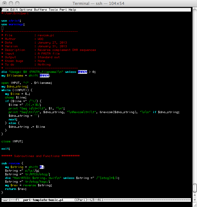
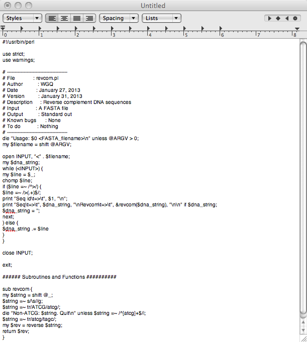
Sample code:#!/usr/bin/perl
use strict;
use warnings;
# ----------------------------------------
# File : extract.pl
# Author : WGQ
# Date : February 20, 2014
# Description : Emmulate glimmer EXTRACT program
# Input : A FASTA file with 1 DNA seq and coord file from LONG-ORF
# Output : A FASTA file with extracted DNA sequences
# ----------------------------------------
die "Usage: $0 <FASTA_file> <coord_file>\n" unless @ARGV > 0;
my ($fasta_file, $coord_file) = @ARGV;
# Read DNA sequence file
open FASTA, "<" . $fasta_file;
my $seq_id;
my $dna_string = "";
my $count_seq = 0;
while (<FASTA>) {
my $line = $_;
chomp $line;
if ($line =~ /^>(.+)$/) {
$seq_id = $1;
$count_seq++;
next;
} else {
$dna_string .= $line
}
}
close FASTA;
die "More than one DNA sequence found. Quit.\n" if $count_seq > 1;
# Read COORD file & extract sequences
open COORD, "<" . $coord_file;
while (<COORD>) {
my $line = $_;
chomp $line;
next unless $line =~ /^s*(\d+)\s+(\d+)\s+(\S+)\s+(\S+)\s+\S+\s*/; # extract data using regex & skip all other lines
my ($id, $cor1, $cor2, $frame) = ($1, $2, $3, $4);
print ">$id\n";
print &orf_seq($cor1, $cor2, $frame), "\n";
}
close COORD;
exit;
###### Subroutines and Functions ####################
sub orf_seq {
my ($x, $y, $fr) = @_;
my $orf;
if ($x < $y) { # positive frame
$orf = substr($dna_string, $x - 1, $y - $x + 1); # substr uses zero-based coord system
} else { # negative frame
$orf = substr($dna_string, $y - 1, $x - $y + 1); # substr uses zero-based coord system
$orf = &revcom($orf);
}
return $orf;
}
sub revcom {
my $string = shift @_;
$string =~ tr/atcg/tagc/; # complement if lower cases
$string =~ tr/ATCG/TAGC/; # complement if upper cases
my $rev = reverse $string; # reverse
return $rev;
}
|
Read, Watch, & Respond (5 pts)
{{#ev:youtube|SS-9y0H3Si8|200|left|An introduction to Object-Oriented Programming}} |
February 12 (No Class)
- Lincoln's Birthday
February 19. Genomics (2): BioPerl
- Lecture Slides: File:Session-3-small.pdfSession 3
- Learning goal: (1) Object-Oriented Perl; (2) BioPerl
- In-Class Exercises
Construct and dump a Bio::Seq object
#!/usr/bin/perl -w
use strict;
use lib '/data/biocs/b/bio425/bioperl-live';
use Bio::Seq;
use Data::Dumper;
my $seq_obj = Bio::Seq->new( -id => "ospC", -seq =>"tgtaataattcaggaaaaga" );
print Dumper($seq_obj);
exit;
Apply Bio::Seq methods:
my $seq_rev=$seq_obj->revcom()->seq(); # reverse-complement & get sequence string
my $eq_length=$seq_obj->length();
my $seq_id=$seq_obj->display_id();
my $seq_string=$seq_obj->seq(); # get sequence string
my $seq_translate=$seq_obj->translate()->seq(); # translate & get sequence string
my $subseq1 = $seq_obj->subseq(1,10); # subseq() returns a string
my $subseq2= $seq_obj->trunc(1,10)->seq(); # trunc() returns a truncated Bio::Seq object
- Challenge 1: Write a BioPerl-based script called "bioperl-exercise.pl". Start by constructing a Bio::Seq object using the "mystery_seq1.fas" sequence. Apply the
trunc()method to obtain a coding segment from base #308 to #751. Reverse-complement and then translate the segment. Output the translated protein sequence.
#!/usr/bin/perl -w
use strict;
use lib '/data/biocs/b/bio425/bioperl-live';
use Bio::Seq;
my $seq_obj = Bio::Seq->new( -id => "mystery_seq", -seq =>"tgtaataattcaggaaaaga.............." );
print $seq_obj->trunc(308, 751)->revcom()->translate()->seq(), "\n";
exit;
- Challenge 2. Re-write the above code using Bio::SeqIO to read the "mystery_seq1.fas" sequence and output the protein sequence.
#!/usr/bin/perl -w
use strict;
use lib '/data/biocs/b/bio425/bioperl-live';
use Bio::SeqIO;
die "$0 <fasta_file>\n" unless @ARGV == 1;
my $file = shift @ARGV;
my $input = Bio::Seq->new( -file => $file, -format =>"fasta" );
my $seq_obj = $input->next_seq();
print $seq_obj->trunc(308, 751)->revcom()->translate()->seq(), "\n";
exit;
| Assignment #3 (Finalized 2/20, 9pm) |
|---|
BioPerl exercises
Sample code: #!/usr/bin/perl
use strict;
use warnings;
use lib '/data/biocs/b/bio425/bioperl-live';
use Bio::SeqIO;
# ----------------------------------------
# File : extract.pl
# Author : WGQ
# Date : February 20, 2014
# Description : Emulate glimmer EXTRACT program
# Input : A FASTA file with 1 DNA seq and coord file from LONG-ORF
# Output : A FASTA file with translated protein sequences
# ----------------------------------------
die "Usage: $0 <FASTA_file> <coord_file>\n" unless @ARGV > 0;
my ($fasta_file, $coord_file) = @ARGV;
my $input = Bio::SeqIO->new(-file=>$fasta_file, -format=>'fasta'); # create a file handle to read sequences from a file
my $output = Bio::SeqIO->new(-file=>">$fasta_file".".out", -format=>'fasta'); # create a file handle to output sequences into a file
my $seq_obj = $input->next_seq();
# Read COORD file & extract sequences
open COORD, "<" . $coord_file;
while (<COORD>) {
my $line = $_;
chomp $line;
next unless $line =~ /^(\d+)\s+(\d+)\s+(\d+)\s+\S+\s+\S+\s*/; # extract data using regex & skip all other lines
my ($seq_id, $cor1, $cor2) = ($1, $2, $3);
if ($cor1 < $cor2) {
$output->write_seq($seq_obj->trunc($cor1, $cor2)->translate());
} else {
$output->write_seq($seq_obj->trunc($cor2, $cor1)->revcom()->translate());
}
}
close COORD;
exit;
|
Read & Respond
|
February 26. Genomics (3). Homology searching with BLAST
- Lecture Slides: File:Session-4-small.pdfSession 4
- Learning goals: Homology, BLAST, & Alignments
- In-Class Challenge. Compose a BioPerl-based script ("translation.pl") for translating a DNA sequence. Input: a DNA file in FASTA (e.g., "bio425/data/TenSeq.nuc") . Output: protein sequences in FASTA. Once the code is working, add a regular expression to skip and warn users for any translated sequence that doesn't start with with a start codon ("ATG" or "TTG"), or doesn't end with a stop codon ("TAG", "TAA", "TGA"), or contains internal stop codons.
- BLAST tutorial 1. A single unknown sequence against a reference genome
cp ../../bio425/data/GBB.pep ~/. # Copy the reference genome
cp ../../bio425/data/unknown.pep ~/. # Copy the query sequence
makeblastdb -in GBB.pep -dbtype prot -parse_seqids -out ref # make a database of reference genome
blastp -query unknown.pep -db ref # Run simple protein blast
blastp -query unknown.pep -db ref -evalue 1e-5 # filter by E values
blastp -query unknown.pep -db ref -evalue 1e-5 -outfmt 6 # concise output
blastp -query unknown.pep -db ref -evalue 1e-5 -outfmt 6 | cut -f2 > homologs-in-ref.txt # save a list of homologs
blastdbcmd -db ref -entry_batch homologs-in-ref.txt > homologs.pep # extract homolog sequences- BLAST tutorial 2. Find homologs within the new genome itself
cp ../../bio425/data/N40.pep ~/. # Copy the unknown genome
makeblastdb -in N40.pep -dbtype prot -parse_seqids -out N40 # make a database of the new genome
blastp -query unknown.pep -db N40 -evalue 1e-5 -outfmt 6 | cut -f2 > homologs-in-N40.txt # find homologs in the new genome
blastdbcmd -db N40 -entry_batch homologs-in-N40.txt >> homologs.pep # append to homolog sequences- BLAST tutorial 3. Multiple alignment & build a phylogeny
../../bio425/bin/muscle -in homologs.pep -out homologs.aln # align sequences
cat homologs.aln | tr ':' '_' > homologs2.aln
../../bio425/bin/FastTree homologs2.aln > homologs.tree # build a gene tree
../../bio425/figtree & # view tree (works only in the lab; install your own copy if working remotely)- BLAST tutorial 4. Annotate the entire genome
blastp -query N40.pep -db ref -evalue 1e-5 -outfmt 6 > blast.fwd # foward blast
blastdbcmd -db ref -entry all > ref.pep
blastp -query ref.pep -db N40 -evalue 1e-5 -outfmt 6 > blast.rev # reverse blast| Assignment #4 (Finalized Sat 3/1) |
|---|
BLAST exercise (5 pts)
|
BioPerl exercise (5 pts)
#!/usr/bin/perl -w
use strict;
use lib '/data/biocs/b/bio425/bioperl-live';
use Bio::SeqIO;
die "Usage: $0 <a FASTA file> <id>\n" unless @ARGV == 2;
my ($file, $id) = @ARGV;
my $in = Bio::SeqIO->new(-file=>$file, -format=>'fasta');
my $found = 0; # used to record if sequence is found or not (boolean)
while(my $seqobj=$in->next_seq()) {
    my $seq_id = $seqobj->display_id();
    if ($seq_id eq $id) {
        print ">$seq_id\n", $seqobj->seq(), "\n";
        $found = 1;
    }
}
warn "No sequence with ID $id is found\n" unless $found;
exit;
|
Read & Respond (5 pts)
|
March 5: Genomics (4). Molecular phylogenetics
- Lecture Slides:
- Learning goal: how to interpret, build, and test phylogeny
- Perl challenge: Write a BioPerl script ("get-seq-from-gb.pl") to retrieve a sequence from the GenBank. Follow the example in Bio::DB::GenBank. Input: a GenBank accession (e.g., "J00522"). Output: a file in "genbank" format. Note: include this statement:
use lib '/data/biocs/b/bio425/perl5';
#!/usr/bin/perl -w
use strict;
use lib '/data/biocs/b/bio425/bioperl-live';
use lib '/data/biocs/b/bio425/perl5';
use Bio::DB::GenBank;
use Bio::SeqIO;
die "Usage: $0 <genbank_accession, e.g., J00522>\n" unless @ARGV == 1;
my $acc = shift @ARGV;
my $gb = Bio::DB::GenBank->new();
my $seq = $gb->get_Seq_by_acc($acc);
my $out = Bio::SeqIO->new(-file=>">" . $acc.".gb", -format=>'genbank');
$out->write_seq($seq);
exit;
- Tutorials
- Tree Quizzes: File:Baum etal05 Quiz.pdfTree Quizzes
- Maximum Parsimony: Exercise 2.4 (pg. 123)
| Assignment #5 (Finalized, 3/7 Friday 9pm) |
|---|
| Phylogeny questions (5 pts) Referring to the tree at right, answer the following questions. Explain your answer.
|
| BLAST and phylogeny exercise (5 pts) Identify all homologs of BBA68 in the ref and N40 genomes using BLASTp. Construct a phylogeny of BBA68 homologs using MUSCLE and FastTree. View and edit the tree using FigTree (download and install your own copy if you are not using the lab computers). Root the tree on the mid-point by following the right-side panel "Trees"->"Root tree"->"midpoint". Based on the phylogeny, identify N40 orthologs of the following B31 genes: BBA68, BBA69, BBA71, BBA72, and BBA73. (Bonus +2 pts) What are the two possible evolutionary mechanisms that there is no ortholog of BBA70 in the N40 genome? Your answer should consist of the following parts:
|

March 12: Putting it together: Annotating a new genome
- Review: File:Session-6-small.pdfReview slides
- Annotate a genome in class: Claim your genome
- No homework assignments this week. Review ALL of your previous assignments
March 19. Midterm Practicum
10:10-12 (No computer access)
March 26 (No Class; Do Assignment #6)
| Assignment #6 (Finalized on Friday, 3/21) |
|---|
Perl/BioPerl Exercises (5+5 pts)
#!/usr/bin/perl -w
use strict;
use lib '/data/biocs/b/bio425/bioperl-live';
use Bio::Tools::SeqStats;
use Bio::SeqIO;
use Data::Dumper;
die "Usage: $0 <fasta>\n" unless @ARGV == 1;
my $filename = shift @ARGV;
my $in = Bio::SeqIO->new(-file=>$filename, -format=>'fasta');
my $seqobj = $in->next_seq();
my $seq_stats = Bio::Tools::SeqStats->new($seqobj);
my $monomers = $seq_stats->count_monomers();
my $codons = $seq_stats->count_codons();
print Dumper($monomers, $codons);
exit;
|
Read & Respond (5 pts)
|
April 2: Transcriptome (1): Univariate statistics
- Learning goals: 1. Microarray technology; 2. Introduction to R
- Lecture Slides:
- R Tutorial 1
- Set a working directory
- Using a Linux terminal, make a directory called
R-work - Start R:
Type "R" on terminal prompt and hit return(Note: This link works only if you use computers in the 1000G lab. Install and use your own R & R Studio for homework assignments) - Find working directory with
getwd() - Change working directory with
setwd("~/R-work")
- Using a Linux terminal, make a directory called
- The basic R data structure: Vector
- Construct a character vector with
c.vect=c("red", "blue", "green", "orange", "yellow", "cyan") - Construct a numerical vector with
n.vect=c(2, 3, 6, 10, 1, 0, 1, 1, 10, 30) - Construct vectors using functions
n.seq1=1:20n.seq2=seq(from=1, to=20, by=2)n.rep1=rep(1:4, times=2)n.rep2=rep(1:4, times=2, each=2)
- Use built-in help of R functions:
?seqorhelp(seq) - Find out data class using the class function:
class(c.vect)
- Construct a character vector with
- Access vector elements
- A single value:
n.vect[2] - A subset:
n.vect[3:6] - An arbitrary subset:
n.vect[c(3,7)] - Exclusion:
n.vect[-8] - Conditional:
n.vect[n.vect>5]
- A single value:
- Apply functions
- Length:
length(n.vect) - Range:
range(n.vect); min(n.vect); max(n.vect) - Descriptive statistics:
sum(n.vect); var(n.vect); sd(n.vect) - Sort:
order(n.vect). How would you get an ordered vector of n.vect? [Hint: use?orderto find the return values] - Arithmetics:
n.vect +10; n.vect *10; n.vect / 10
- Length:
- Quit an R session
- Click on the "History" tab to review all your commands
- Save your commands into a file by opening a new "R Script" and save it as
vector.R - Save all your data to a default file .RData and all your commands to a default file ".Rhistory" with
save.image() - Quit R-Studio with
q()
- R tutorial 2
- Start a new R studio session and set working directory to
~/R-work - Generate a vector of 100 normal deviates using
x.ran=rnorm(100) - Visualize the data distribution using
hist(x.ran) - Explore help file using
?help; example(hist) - How to break into smaller bins? How to add color? How to change x- and y-axis labels? Change the main title?
- Test if the data points are normally distributed.[Hints: use qqnorm() and qqline()]
- Save a copy of your plot using "Export"->"Save Plot as PDF"
- R tutorial 3
- Using a Linux terminal, make a copy of breast-cancer transcriptome file
/data/biocs/b/bio425/data/ge.datin your R working directory - Start a new R studio session and set working directory to
~/R-work - Read the transcriptome file using
ge=read.table("ge.dat", header=T, row.names=1, sep="\t")- What is the data class of
ge? - Access data frame. What do the following commands return?
ge[1,]; ge[1:5,]; ge[,1]; ge[,1:5]; ge[1:5, 1:5] - Apply functions:
head(ge); tail(ge); dim(ge)
- What is the data class of
- Save a copy of an object:
ge.df=ge. - Transform the transcriptome into a numerical matrix for subsequent operations:
ge=as.matrix(ge) - Test if the expression values are normally distributed.
- Save and quit the R session
- In class challenge: Replicate normalization in Figure 4.8 (pg 208)
| Assignment #7 (Finalized on Sat, 4/5) |
|---|
|
April 9: Transcriptome (2): Bi- and Multi-variate statistics
- Learning goal: (1) multivariate clustering analysis; (2) Classification of breast-cancer subtypes
- Lecture slides:
- Tutorial 1. Gene filtering
- Open a new R Studio session and set working directory to R-work
- Load the default workspace and plot a histogram of the gene expression using
hist(ge, br=100). Answer the following questions:- Make sure
geis a matrix class. If not, review the last session on how to make one - What is the range of gene expression values? Minimum? Maximum?
range(ge); min(ge); max(ge)
- Are these values normally distributed? Test using
qqnormandqqline. - If not, which data range is over-represented? Why?
Low gene expression values are over-represented, because most genes are NOT expressed in a particular cell type/tissue.
- Make sure
- Discussion Questions:
- What does each number represent?
log2(cDNA)
- Why is there an over-representation of genes with low expression values?
Because most genes are not expressed in these cancer cells
- How to filter out these genes?
Remove genes that are expressed in low amount in these cells, by using the function pOverA (see below)
- How to test if the filtering is successful or not?
Run qqnorm() and qqline()
- What does each number represent?
- Remove genes that do not vary significantly among breast-cancer cells
- Download the genefilter library from BioConductor using the following code
source("http://bioconductor.org/biocLite.R"); biocLite("genefilter") - Load the genefilter library with
library(genefilter) - Create a gene-filter function:
f1=pOverA(p=0.5, A=log2(100)). What is thepOverAfunction?Remove genes expressed with lower than log2(100) amount in half of the cells
- Obtain indices of genes significantly vary among the cells:
index.retained=genefilter(ge, f1) - Get filtered expression matrix:
ge.filtered=ge[index.retained, ]. How many genes are left?dim(ge.filtered)
- Download the genefilter library from BioConductor using the following code
- Test the normality of the filtered data set
- Plot with
hist(); qqnorm(); and qqline(). Are the filtered data normally distributed? - Plot with
boxplot(ge.filtered). Are expression levels distributed similarly among the cells?
- Plot with
- Tutorial 2. Select genes vary the most in gene expression
- Explore the function
mad. What are the input and output?Input: a numerical array. Output: median deviation
- Calculate mad for each gene:
mad.ge=apply(ge.filtered, MARGIN=1, FUN=mad) - Obtain indices of the top 100 most variable genes:
mad.top=order(mad.ge, decreasing=T)[1:100] - Obtain a matrix of most variable genes:
ge.var=ge.filter[mad.top,]
- Part 3. Classify cancer subtypes based on gene expression levels
- Discussion Questions:
- How would you measure the difference between a one-dimensional variable?
d=|x1-x2|
- How would you measure the difference between a two-dimensional variable?
d=|x1-x2|+|y1-y2|
- How would you measure the Euclidean difference between a three-dimensional variable?
d=|x1-x2|+|y1-y2|+|z1-z2|
- How would you measure the Euclidean difference between a multi-dimensional variable?
d=SQRT(sum([xi-xj]^2))
- To measure similarities between cells based on their gene expression values, is it better to use Euclidean or correlation distances?
Correlational distance measures similarity in trends regardless of magnitude.
- How would you measure the difference between a one-dimensional variable?
- Calculate correlation matrix between cells:
cor.cell=cor(ge.var) - Calculate correlation matrix between genes:
cor.gene=cor(t(ge.var))What does the t() function do?transposition (turn rows into columns and columns into rows)
- Obtain correlational distances between cells:
dg.cell=as.dendrogram(hclust(as.dist(1-cor.cell))) - Obtain correlational distances between genes:
dg.gene=as.dendrogram(hclust(as.dist(1-cor.gene))) - Plot a heat map:
heatmap(ge.var, Colv=dg.cell, Rowv=dg.gene)
| Assignment #8 (Finalized 4/15) |
|---|
|
April 16 (No Class)
- Spring Break
April 23: Transcriptome (3). RNA-SEQ Analysis
- Learning goal: RNA-SEQ pipeline
- Lecture slides:
- Read data source GSE32038
- Tutorial 1. Visualize expression levels
gene.fpkm=read.table("../../bio425/data/genes.fpkm_tracking", head=T, sep="\t")
dim(gene.fpkm)
head(gene.fpkm)
fpkm=gene.fpkm[which(gene.fpkm$C1_status=='OK' & gene.fpkm$C2_status=='OK'),] # filter low-quality values
hist(log10(fpkm$C1_FPKM), br=100)
plot(density(log10(fpkm$C1_FPKM)))
plot(log10(fpkm$C1_FPKM), log10(fpkm$C2_FPKM))
fpkm.m=log2(fpkm$C1_FPKM) + log2(fpkm$C2_FPKM)
fpkm.a=log2(fpkm$C1_FPKM) - log2(fpkm$C2_FPKM)
plot(fpkm.m, fpkm.a)
- Tutorial 2. Test differential gene expressions
gene=read.table("~/bio-425-spring-2014/cuff_out/gene_exp.diff", header=T, sep="\t")
dim(gene)
head(gene)
gene.ok=gene[which(gene$status=='OK'),] # filter
gene.sig=gene.ok[which(gene.ok$significant=="yes"),] # select significant genes
plot(gene.ok$log2.fold_change., -log10(gene.ok$q_value)) # volcano plot
plot(gene.ok$log2.fold_change., -log10(gene.ok$q_value), col=gene.ok$significant)
| Assignment #9 (Finalized 4/25, Friday 5pm) |
|---|
|
April 30: Population Analysis (1)
- Learning goals: (1) SNP analysis (single-locus), (2) haplotype analysis (multiple loci)
- Lecture slides:
Tutorial. Linkage disequilibrium. Install and use the R package "genetics". Understand genotype, individual, SNP site, HWE, LD table
source('http://www.bioconductor.org/biocLite.R')
biocLite("genetics")
library(genetics)
data=read.csv("example_data.csv") # copy the file from "bio425/data" to R-work first
data=makeGenotypes(data)
HWE.test(data$c104t) # Hardy-Weinberg equilibrium
ld=LD(data) # pairwise D', r, and p-values
LDtable(ld) # visualize LD table
summary(lm( DELTA.BMI ~ homozygote(c104t,'C') + allele.count(a1691g, 'G') + c2249t, data=data)) # linear regression
#Challenge: Read the output file from the PERL script above & calculate LD table. Verify with the alignment.
Tutorial. Contingency Table tests (Analysis of Frequencies & Proportions)
fisher.test(matrix(c(9,1,2,4), nrow=2))
chisq.test(matrix(c(9,1,2,4), nrow=2), simulate.p.value=T) # ch-squared test with simulated p value
| Assignment #10 (Finalized on Friday 5/2/14 12 noon) |
|---|
|
May 7: Population Analysis (2)
- Learning goals: Case-Control studies for gene mapping
- Lecture slides:
- Tutorial: Descriptive genetic statistics of a population. Copy and paste the following BioPerl code as "popstat.pl". Run the code with the "bio425/data/snp.dat" and "exercise-3-1.aln" as the input files. Annotate the statements. Modify the code to print the haplotypes consisting of 1st and 2nd SNP sites. Analysis output (LDtable) using the R package "genetics".
#!/usr/bin/perl
# Input: CLUSTALW alignment
# Output: Haplotypes
use warnings;
use strict;
use lib '/data/biocs/b/bio425/bioperl-live';
use Bio::AlignIO;
use Bio::PopGen::Utilities;
use Bio::PopGen::Population;
die "Usage: $0 <alignment_file>\n" unless @ARGV > 0;
my $file = shift @ARGV; # store filename in variable $file
my $in = Bio::AlignIO->new(-file=>$file, -format=>'clustalw'); # read alignment from the file
my $aln = $in->next_aln(); # get an alignment object
my $pop = Bio::PopGen::Utilities->aln_to_population(
    -alignment           => $aln,
    -include_monomorphic => 0,
    -site_model          => 'all'
    ); # create a population object from an alignment object

for my $ind ($pop->get_Individuals()) { # for each individual
  print $ind->unique_id(), "\t"; # print id
  for my $name ( sort {$a <=> $b} $pop->get_marker_names() ) { # for each SNP site, sorted numerically by positions
    my @genotypes = $ind->get_Genotypes(-marker => $name); #  get genotype as an array
    my $geno = shift @genotypes;  # get genotype at this SNP site
    my @alleles = $geno->get_Alleles(); # get alleles at this SNP site
    my $allele = shift @alleles; # get a single allele
    print $allele;
  }
  print "\n";
}
exit;
May 14: Final Review
- Review slides:
- BioPerl exercises: Modify the above code to (1) calculate heterozygosity at all SNP sites; (2) output 2-loci haplotype frequencies
- Free registration for One-Day (May 29, Thursday) Bioinformatics Symposium at Hunter: Extra credits for full-day attendance
- Teacher's evaluation
May 21: Final Exam
- Exam has been posted on Sat 5/17 4pm:
Note: Print & submit the first 3 pages (there is NO need to print or submit the other pages)
- Due by 5pm, Wed May 21, 2014, @ HN839 (my office)
- Reminder: Teacher's evaluation
General Information
Course Description
- Background: Biomedical research is becoming a high-throughput science. As a result, information technology plays an increasingly important role in biomedical discovery. Bioinformatics is a new interdisciplinary field formed between molecular biology and computer science.
- Contents: This course will introduce both bioinformatics theories and practices. Topics include: database searching, sequence alignment, molecular phylogenetics, structure prediction, and microarray analysis. The course is held in a UNIX-based instructional lab specifically configured for bioinformatics applications.
- Problem-based Learning (PBL): For each session, students will work in groups to solve a set of bioinformatics problems. Instructor will serve as the facilitator rather than a lecturer. Evaluation of student performance include both active participation in the classroom work as well as quality of assignments (see #Grading Policy).
- Learning Goals: After competing the course, students should be able to perform most common bioinformatics analysis in a biomedical research setting. Specifically, students will be able to
- Approach biological questions evolutionarily ("Tree-thinking")
- Evaluate and interpret computational results statistically ("Statistical-thinking")
- Formulate informatics questions quantitatively and precisely ("Abstraction")
- Design efficient procedures to solve problems ("Algorithm-thinking")
- Manipulate high-volume textual data using UNIX tools, Perl/BioPerl, R, and Relational Database ("Data Visualization")
- Pre-requisites: This 3-credit course is designed for upper-level undergraduates and graduate students. Prior experiences in the UNIX Operating System and at least one programming language are required. Hunter pre-requisites are CSCI132 (Practical Unix and Perl Programming) and BIOL300 (Biochemistry) or BIOL302 (Molecular Genetics), or permission by the instructor. Warning: This is a programming-based bioinformatics course. Working knowledge of UNIX and Perl is required for successful completion of the course.
- Textbook: Gibson & Muse (2009). A Primer of Genome Science (Third Edition). Sinauer Associates, Inc.
- Academic Honesty: Hunter College regards acts of academic dishonesty (e.g., plagiarism, cheating on examinations, obtaining unfair advantage, and falsification of records and official documents) as serious offenses against the values of intellectual honesty. The College is committed to enforcing the CUNY Policy on Academic Integrity and will pursue cases of academic dishonesty according to the Hunter College Academic Integrity Procedures.
Grading Policy
- Treat assignments as take-home exams. Student performance will be evaluated by weekly assignments and projects. While these are take-home projects and students are allowed to work in groups and answers to some of the questions are provided in the back of the textbook, students are expected to compose the final short answers, computer commands, and code independently. There are virtually an unlimited number of ways to solve a computational problem, as are ways and personal styles to implement an algorithm. Writings and blocks of codes that are virtually exact copies between individual students will be investigated as possible cases of plagiarism (e.g., copies from the Internet, text book, or each other). In such a case, the instructor will hold closed-door exams for involved individuals. Zero credits will be given to ALL involved individuals if the instructor considers there is enough evidence for plagiarism. To avoid being investigated for plagiarism, Do NOT copy from others or let others copy your work.
- Submit assignments in Printed Hard Copies. Email attachments will NOT be accepted. Each assignment will be graded based on timeliness (10%), whether executable or having major errors (50%), algorithm efficiency (10%), and readability in programming styles (30%, see #Assignment Expectations).
- The grading scheme
- Assignments (100 pts): 10 exercises.
- Mid-term (50 pts).
- Final Project (50 pts)
- Classroom performance (50 pts): Active engagement in classroom exercises and discussions
- Attendance (50 pts): 1 unexcused absences = 40; 2 absences = 30; More than 2 = 0.
Assignment Expectations
- Use a programming editor (e.g., vi or emacs) so you could have features like automatic syntax highlighting, indentation, and matching of quotes and parenthesis.
- All PERL code must begin with "use strict; and use warnings;" statements. For each assignment, unless otherwise stated, I would like the full text of the source code. Since you cannot print using the text editor in the lab (even if you are connected from home), you must copy and paste the code into a word processor or a local text editor. If you are using a word processor, change the font to a fixed-width/monospace font. On Windows, this is usually Courier.
- Also, unless otherwise stated, both the input and the output of the program must be submitted as well. This should also be in fixed-width font, and you should label it in such a way so that I know it is the program's input/output. This is so that I know that you've run the program, what data you have used, and what the program produced. If you are working from the lab, one option is to email the code to yourself, change the font, and then print it somewhere else as there is no printer in the lab.
- Recommended Style
- Bad Style
Useful Links
Unix Tutorials
- A very nice UNIX tutorial (you will only need up to, and including, tutorial 4).
- FOSSWire's Unix/Linux command reference (PDF). Of use to you: "File commands", "SSH", "Searching" and "Shortcuts".
Perl Help
- Professor Stewart Weiss has taught CSCI132, a UNIX and Perl class. His slides go into much greater detail and are an invaluable resource. They can be found on his course page here.
- Perl documentation at perldoc.perl.org. Besides that, running the perldoc command before either a function (with the -f option ie, perldoc -f substr) or a perl module (ie, perldoc Bio::Seq) can get you similar results without having to leave the terminal.
Regular Expression
Bioperl
- BioPerl's HOWTOs page.
- BioPerl-live developer documentation. (We use bioperl-live in class.)
- Yozen's tutorial on installing bioperl-live on your own Mac OS X machine. (Let me know if there are any issues!).
- A small table showing some methods for BioPerl modules with usage and return values.
SQL
- SQL Primer, written by Yozen.
R Project
- Install location and instructions for Windows
- Install location and instructions for Mac OS X
- Install R-Studio
- For users of Ubuntu/Debian:
sudo apt-get install r-base-core
Utilities
- An RSS button extension for chrome. Can add feeds to Google Reader and others.
- A similar extension which adds a "Live bookmarks"-like feature to Chrome (like Firefox's RSS bookmarks).
Other Resources
- Information Theory Primer by Thomas D. Schneider. Useful in understanding sequence logo maps.
© Weigang Qiu, Hunter College, Last Update ~~