QuBi/modules/biol303

Bioinformatics Lab: Exploration of Gene Expression in Dictyostelium species

Figure 1. Development of Dictyostelium (M. Grimson, R. Blanton, Texas Tech University)

Objectives

Understand the RNA-SEQ technology and its use in genome-wide identification of gene functions.
Be able to identify co-expressed and co-repressed genes based on time-course gene expression data.

Lab Report Grading Policy

Introduction (1 pts): Define transcriptome. List key steps in RNA-SEQ technology. Describe advantages of high-throughput technologies in comparison with traditional gene-by-gene approaches of studying gene function. Your statements are not to be copied from the Lab Manual.

Materials and Methods (1 pts): Describe experimental procedures of the study that have produced these gene expression data by reading this paper and this experimental report. Answer the following questions:

Name of the two species used in experiments
How many genes were measured for their expression levels?
How many time points, developmental stages, and cell types have been tested?

Results (5 pts)

Table 2 (annotation for 15 genes)
Expression profiles (screen capture for 15 genes)
Table 4 (correlation coefficients)
Heat map of 15 genes (screen capture)

Discussion (2 pts): Answer the four discussion questions.

Summary/Conclusion (1 pt): A sentence or two will suffice.

References (1 pt): Credit is given for pertinent references obtained from sources other than the Lab Manual.

Introduction

Figure 2. a) Results from four individual Northern blots examining four different genes and measuring mRNA production over time, as indicated. b) Results from a series of microarrays for the same four genes of interest. Note the color scale on the bottom of b), where bright green indicates a 20-fold repression and bright red indicates a 20-fold induction. Black indicates no change in transcription. (Source: Campbell & Heyer. (2003). Discovering Genomics, Proteomics, & Bioinformatics. Pearson Education, Inc.)

Figure 3. A typical RNA-Seq experiment. Briefly, long RNAs are first converted into a library of cDNA fragments through either RNA fragmentation or DNA fragmentation. Sequencing adaptors (blue) are subsequently added to each cDNA fragment and a short sequence is obtained from each cDNA using high-throughput sequencing technology. The resulting sequence reads are aligned with the reference genome or transcriptome, and classified as three types: exonic reads, junction reads and poly(A) end-reads. These three types are used to generate a base-resolution expression profile for each gene, as illustrated at the bottom; a yeast ORF with one intron is shown. (Source: Wang, Gerstein, and Snyder (2009)). The expression level of a gene is measured by its FPKM, which stands for fragments per kilobase of total gene length per million mapped reads. In essence, FPKM is the amount of short reads mapped to a gene normalized by the gene length and the total number of reads generated from an experiment. The normalization by gene length and total reads makes it possible to compare expression levels across genes as well as among experiments.

Gene expression is the transcription of a DNA template into RNA molecules, some of which are eventually translated into proteins. In a multicellular organism, the subset of genes that are expressed defines and gives rise to a specific tissue or cell type. In this laboratory exercise, we will use bioinformatics techniques to identify genes up- and down-regulated in Dictyostelium during its development from a unicellular stage to a multi-cellular stage.

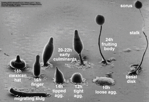
Due to its unique mode of development (Figure 1), Dictyostelium is an important model organism for the study of how multicellular organisms evolved from unicellular ones. It is also a key disease model for understanding cancer, especially regarding the mechanism of cell migration, chemotaxis, and metastasis.

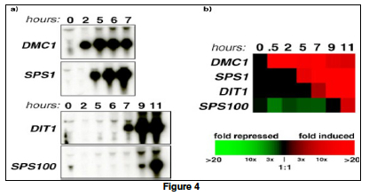
Traditionally, gene expressions are studied one gene at a time using blotting techniques. For example, in a Northern Blot experiment (Figure 2a), the whole messenger RNA (mRNA) content of a cell is extracted and loaded on a solid gel slab. Different mRNA molecules are then separated using electrophoresis and transferred to a nitrocellulose sheet. To identify if a gene is expressed, a radioactively (or fluorescently) labeled oligonucleotide probe that is specific to the gene sequence is applied to the sheet. If the gene is expressed, the probe will hybridize with a specific mRNA molecule and a black band will appear on an Xray film. Other blotting techniques for detecting gene expression include Southern Blot, in which mRNAs in a cell are reverse transcribed to their complementary DNA (cDNA) before being hybridized with gene-specific oligo-nucleotide probes. In a Western Blot experiment, the protein product (instead of the mRNA intermediate) of a gene is probed using antibodies (instead of the oligonucleotide probes).

After the genomic revolution since the 1990s, it became possible to study the expression of all genes in a cell at once using high-throughput techniques. Detecting the expression profiles of a whole genome was made possible by the availability of the whole genome sequences of bacteria, yeasts, and humans. The DNA microarray (Figure 2b) is one such high throughput technique. In contrast to the Northern Blot technique in which the mRNA sample is fixed on a nylon sheet, nucleotide probes for all genes are fixed on a glass slide, creating a “gene chip”. The cellular mRNAs are reverse transcribed into cDNAs labeled with fluorescent dyes, which are then hybridized with the gene chips. After the unattached cDNAs are washed away, the fluorescent intensity remains at each probe location is measured as an indication of the amount of mRNA transcribed from each gene in a genome. The entire cellular RNA content transcribed from a genome is called a transcriptome. Each DNA microarray reading is therefore essentially a snap-shot of the whole genome expression profile of a cell at a particular physiological stage. It is no longer necessary to know or decide beforehand candidate genes to be targets of exploration, as in the traditional blotting techniques.

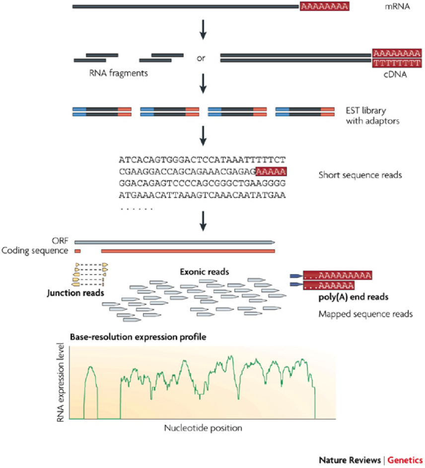
Most recently, direct sequencing of the whole mRNA content of a cell using the so-called RNA-SEQ technology (Figure 3) provides an alternative and even more accurate way of obtaining the transcriptome of a cell. Unlike the microarray technology, the RNA-SEQ technology allows de novo discovery of transcribed genes since it does not rely on a pre-defined DNA probes. Another major advantage of the RNA technology is its ability to detect splice variants, which are differentially spliced exons of the same gene.

These high-throughput technologies, however, create new technical challenges of their own. The main challenge is the analysis of the huge amount of data resulting from each microarray or sequencing experiment. First, data from high-throughput experiments need computer-assisted data processing and analysis. Second, statistical analysis and testing become essential tools for the discovery and exploration of gene functions, e.g., finding co-expressed genes.

Procedures

HINT: Start a WORD or PowerPoint file as your personal lab notebook. Using this file, you could copy and paste gathered information as well as write notes to yourself.

Understand the design of an RNA-SEQ experiment using NCBI GEO database

Name and describe the two species tested in experiments
How many genes were measured for their expression levels for each species?
How many time points, developmental stages, and cell types have been tested for expression differences?
How many replicates for each developmental stage?

Search for gene information using DictyBase

Select at least five genes from each of 3 gene groups in Table 1
For each of the five genes, search its annotation in DictyBase by copying & pasting the ID in the search box (top right) and click "Search All"
Collect the gene information and make a table by following the example in Table 2

Table 1. Gene lists
Gene Group	DictyBase IDs
Group A	DDB_G0267376 DDB_G0276887 DDB_G0286385 DDB_G0278077 DDB_G0285425 DDB_G0283385 DDB_G0274569 DDB_G0269108 DDB_G0291372 DDB_G0269124 DDB_G0284331 DDB_G0280047 DDB_G0283907 DDB_G0292436 DDB_G0289329 DDB_G0289075 DDB_G0288677 DDB_G0277215 DDB_G0275687 DDB_G0280961 DDB_G0281381 DDB_G0287291 DDB_G0286121 DDB_G0288041 DDB_G0292266 DDB_G0281387
Group B	DDB_G0277823 DDB_G0292460 DDB_G0271976 DDB_G0278539 DDB_G0288273 DDB_G0281677 DDB_G0285277 DDB_G0286117 DDB_G0291526 DDB_G0290141 DDB_G0271668 DDB_G0283597 DDB_G0283741 DDB_G0272893 DDB_G0268302 DDB_G0289593 DDB_G0284093 DDB_G0285759 DDB_G0281469 DDB_G0267604 DDB_G0293700 DDB_G0281565 DDB_G0273191 DDB_G0285881 DDB_G0276871 DDB_G0286399 DDB_G0275881 DDB_G0286075 DDB_G0283275 DDB_G0292388 DDB_G0293742
Group C	DDB_G0275703 DDB_G0282247 DDB_G0269624 DDB_G0278867 DDB_G0280049 DDB_G0290439 DDB_G0269298 DDB_G0293184 DDB_G0293124 DDB_G0274211 DDB_G0269424 DDB_G0282943 DDB_G0286773 DDB_G0282381 DDB_G0269222 DDB_G0293396 DDB_G0271806

Table 2. Gene annotations
DictyBase ID	Gene Name	Gene Product	Description	GO-Molecular Function (MF) (pick one)	GO-Biological Process (BP) (pick one)	GO-Cellular Component (CC) (pick one)	Curator Notes (brief quote)
DDB_G0267376	acrA	adenylate cyclase	contains a cyclase domain, 7 transmembrane helices, a histidine kinase domain, and two receiver domains	adenylate cyclase activity	sporulation resulting in formation of a cellular spore	integral component of membrane	The acrA gene encodes the late developmental stage adenylate cyclase which is essential for spore encapsulation.

Explore expression profiles of individual genes using dictyExpress

Click on the website for dictyExpress and "Run dictyExpress (RNA-seq)."
A tutorial may start if this is your first time using the website. Feel free to do the tutorial. If you do not want to do the tutorial, close the tutorial box.
In the "Experiment and Gene Selection" panel, select "1. D. discoideum vs D. purpurem, Parikh A et.al., D. discoideum." This will select the experiment you read about. Make sure it is highlighted before you do the next steps.
In the "Experiment and Gene Selection" panel, type in a Gene Name from Group A (e.g., acrA) in the area under “Genes.”
Click "Update Selection." A plot should generate in the "Expression Time Course" panel. Screen shot this plot in your notebook/Word Document/PowerPoint file (Hints: Check the "Legend" box to show the gene’s name on the plot. Click the lower right arrow to expand the plot to full screen as needed. You can move around the windows as well by dragging and dropping the window near the title of the window. For example, you can drag and drop the “Expression Time Courses” window to the center of the screen if you wish).
Is this gene up- or down-regulated during development?
Repeat the above for the other genes (15 in total).
Group genes by their similarity in expression profiles. How many such groups can you identify? For each group, describe the pattern and speculate on their functions.

Identify co-regulated genes using correlational distances and cluster analysis

Figure 4. Pearson's r

Figure 5. Calculate r using the Excel function CORREL()

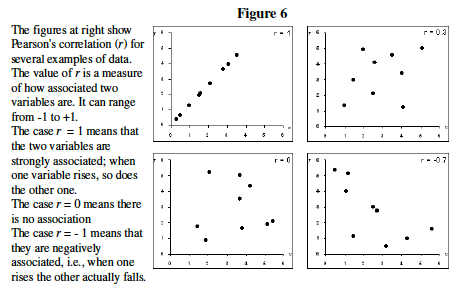
Understand correlation coefficient: Pearson's Correlation Coefficient (r) is a measure of how tightly linked two variables are (Figure 4). Here we will use it to measure the similarity in gene expression profile between two genes. Note that correlation does not necessarily imply causation.
Calculate correlation coefficients using EXCEL
1. Excel easily measures correlation and Pearson's r. Like most calculations in Excel, you simply click on an empty cell, type "=", write a formula, and indicate what range of cells you wish to perform the calculation on. The example in Figure 5 was created by clicking on Cell J3 and entering the formula: =CORREL(B1:H1,B2:H2 ) , which caused the spreadsheet to compare the values in Row 1 and Row 2 and print a correlation value (Pearson's r) in Cell J3 .
2. You will do this for six different pairs of genes in Table 3 (one correlation has to be measured for every possible twosome, i.e. first and second row, first and third row, etc) Write your six pairwise correlation results into Table 4. The correlation of any gene with itself is, of course, perfect, and hence "1". A double dash has been placed in half of the spaces to save you the trouble of writing a result twice. This may take some time, especially if you are unfamiliar with Excel, spreadsheets, or Statistics. Work together and ask someone who can help.
Understand cluster analysis: Watch an HHMI slide presentation on how to group genes and samples by their overall similarity in gene expression levels
In the "Hierarchical Clustering" Panel, choose the "Pearson Correlation" for "Distance Function"
Choose "Average Linkage" for "Linkage" and your choice of color gradient.
Screen-capture the heatmap and record your answers to the following questions
1. What is represented by each row?
2. What is represented by each column?
3. Compare the cluster diagram with the groups you have identified visually. Do they agree with each other?
4. Do three groups of genes (Group A, B, and C; Table 1) form clusters by themselves?

Table 3. Read counts of six genes
DictyBase ID	Gene Name	Hour 00	Hour 04	Hour 08	Hour 12	Hour 16	Hour 20	Hour 24
DDB_G0267376	acrA	47.84401093	220.1386	335.2265	288.9046	333.8650	244.5453	201.6707
DDB_G0267604	mserS	0.563943	3.0999	49.9572	419.2713	2147.4096	1804.1120	4527.1415
DDB_G0268302	rpl38	67.19935935	1.6417	19.8430	5.8377	2.5870	1.5032	4.0678
DDB_G0269108	catB	8600.321169	4904.7794	1429.3452	1503.6344	905.1408	654.8504	995.3257
DDB_G0269222	gefB	3.530691422	285.1393	385.5468	261.5676	251.0168	171.1454	180.7623
DDB_G0269298	gefX	83.30521325	437.0953	227.8182	254.1875	124.2749	70.7291	136.7658

Table 4. Obtain the correlation coefficients using the EXCEL function CORREL
	acrA	mserS	rpl38	catB	gefB	gefX
acrA	1	?	?	?	?	?
mserS	-	1	?	?	?	?
rpl38	-	-	1	?	?	?
catB	-	-	-	1	?	?
gefB	-	-	-	-	1	?
gefX	-	-	-	-	-	1

Discussion Questions

Figure 6. The heat maps represent the patterns of change in standardized mRNA abundance for all the genes in the D. discoideum and the D. purpureum genomes. Each row represents an average of 85 genes and each column represents a developmental time point (hours). The colors represent relative mRNA abundances (see scale). The genes are ordered according to their regulation pattern in each species. The black lines divide the transcripts, from top to bottom, into: down-regulated, intermediate regulation and up-regulated. The dendrograms represent the differences between the transcriptomes at each time point. Source: Parikh et al (2010)

What differences and similarities does a RNA-Seq experiment have with a Northern blot?
Explain how a time-course experiment like this one could be used for discovering gene networks during development.
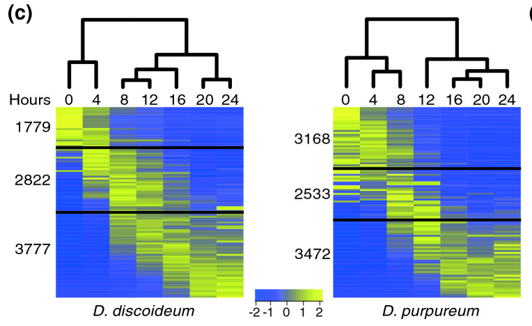
The Parikh et al (2010) paper concludes that developmental pathway genes are conserved in their expression profiles between the two Dictyostelium species. Based on the two heat maps (Figure 6), identify similarities and differences in expression profiles between the two species.
Similar genes (homologs) are found in humans. Do you expect the expression of these genes to be similar during human development? during cancer development?